


Imagine ordering food from an app.
The app tells you, “Your order will arrive in 25 minutes.”
But the delivery actually takes 42 minutes.
The prediction was wrong by 17 minutes.
Now imagine the app makes thousands of these predictions every day. Some are off by two minutes, some by ten, and a few are completely wrong.
If we wanted to improve the prediction system, we would first need a way to answer one simple question:
How wrong are the predictions?
That is exactly what a loss function does in machine learning and deep learning.
A neural network can make a prediction, but it cannot improve simply by knowing that the prediction was “good” or “bad.” It needs a measurable number that tells it how large the mistake was.
That number is called loss.
Why Neural Networks Need a Loss Function
Think about learning to throw a basketball into a hoop.
Your first throw falls two feet short.
On the next attempt, you use more force.
This time, the ball goes slightly too far.
You adjust again.
After several attempts, you begin getting closer to the basket because every miss gives you information about what needs to change.
A neural network learns in a similar way.
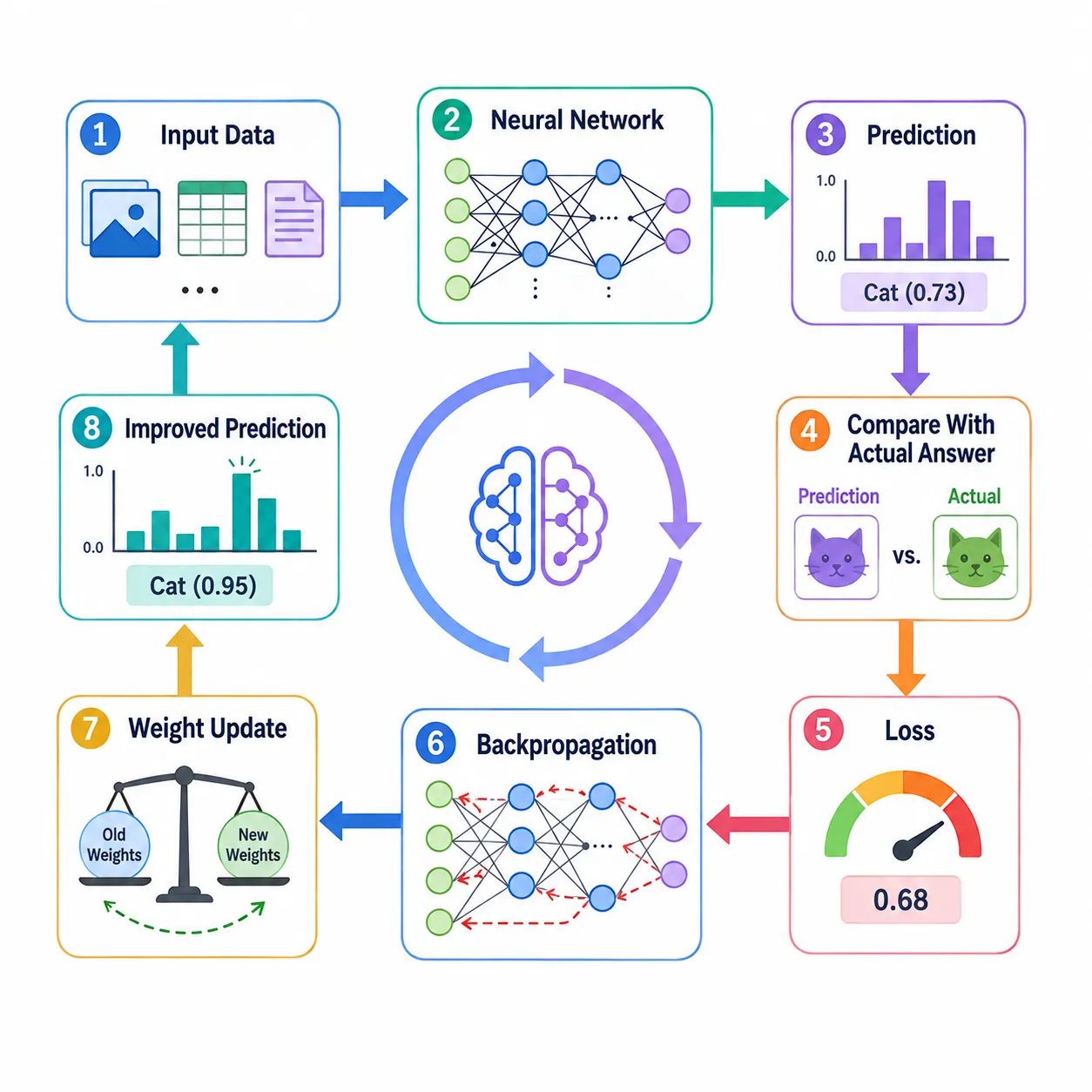
It makes a prediction, compares that prediction with the correct answer, measures the error, and then adjusts its internal weights.
During training, the loss function produces the quantity the model tries to minimize. Frameworks such as Keras describe loss functions in exactly this role: they calculate the value a model should try to reduce during training.
The basic learning cycle looks like this:
Input → Prediction → Compare with actual answer → Calculate loss → Update the network → Try again
This process happens again and again during training.
The goal is not simply to make the loss smaller once. The model tries to find weights that keep producing smaller errors across many training examples.
What Is a Loss Function in Deep Learning?
A loss function in deep learning is a mathematical method used to measure the difference between what a neural network predicted and what the correct answer actually was.
Suppose a model predicts that tomorrow's temperature will be:
Predicted temperature: 30°C
The real temperature turns out to be:
Actual temperature: 34°C
The model missed the target by four degrees.
A loss function converts that mistake into a number the training process can work with.
But there is an important detail.
Not every machine learning problem produces the same type of answer.
Sometimes we predict a number:
House price
Delivery time
Temperature
Sales amount
Electricity demand
These are usually regression problems.
Other times we predict a category:
Spam or not spam
Dog or cat
Fraud or genuine transaction
Positive or negative review
These are classification problems.
Because regression and classification produce different kinds of outputs, they usually need different ways of measuring mistakes.
This is where Mean Squared Error (MSE) and cross-entropy loss enter the picture. MSE is a standard choice for continuous-value regression, while cross-entropy is widely used for classification.
Mean Squared Error (MSE): The Simple Idea
Let's begin with Mean Squared Error, usually shortened to MSE.
MSE asks:
“On average, how far are my numerical predictions from the real values?”
But instead of simply averaging the errors, it squares every error first.
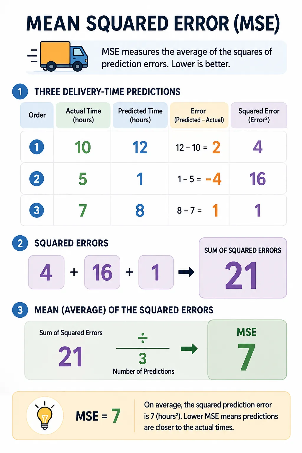
Imagine a model trying to predict the delivery time for three food orders.
For the first order:
Actual time = 30 minutes
Predicted time = 28 minutes
Error = 2 minutes
For the second:
Actual time = 40 minutes
Predicted time = 44 minutes
Error = 4 minutes
For the third:
Actual time = 25 minutes
Predicted time = 24 minutes
Error = 1 minute
Now square those errors:
2² = 4
4² = 16
1² = 1
Add them:
4 + 16 + 1 = 21
Then divide by the number of predictions:
21 ÷ 3 = 7
So the Mean Squared Error is 7.
In simple form:
MSE = Average of (Actual Value − Predicted Value)²
PyTorch describes MSE loss as the mean squared difference between model inputs or predictions and their targets, which matches this basic idea.
Why Does MSE Square the Error?
You may be wondering:
Why square the error? Why not just use the difference?
There are two useful reasons.
First, prediction errors can be positive or negative.
If the real house price is $300,000 and the model predicts $280,000, the difference goes in one direction.
If the model predicts $320,000, the difference goes in the opposite direction.
If we simply added signed errors together, positive and negative errors could cancel each other out.
Squaring removes that problem because every squared value becomes positive.
Second, squaring makes large mistakes much more expensive than small mistakes.
An error of 2 becomes:
2² = 4
But an error of 10 becomes:
10² = 100
So the error is only five times larger before squaring, but its squared penalty is twenty-five times larger.
This gives MSE an important characteristic: it pays extra attention to large prediction mistakes.
A Real-World MSE Example: House Price Prediction
Imagine training a neural network to estimate house prices.
One house is actually worth ₹60 lakh.
Your model predicts ₹59 lakh.
That is a relatively small miss.
Now another house is worth ₹80 lakh, but your model predicts only ₹50 lakh.
That mistake is far more serious.
Because MSE squares errors, the second prediction creates a much larger penalty.
During training, the network receives a stronger signal that something went badly wrong.
This can be useful when large mistakes are especially important.
For example, MSE can make sense when predicting prices, demand, temperatures, energy consumption, or other continuous values where you want the model to strongly react to major misses.
The Hidden Weakness of MSE
The same feature that makes MSE useful can also cause problems.
Because large errors are squared, a single extreme value can have a very strong effect on the total loss.
Imagine most delivery predictions are wrong by only two or three minutes, but one unusual order is delayed by 90 minutes because of a road accident.
That one extreme example could produce a huge squared error.
In other words, MSE is sensitive to outliers. OpenStax also notes that because MSE squares prediction differences, larger errors receive heavier penalties.
That does not make MSE a bad loss function.
It simply means you should understand what kind of mistakes your data contains before choosing it.
And this leads us to the bigger question:
If MSE works so naturally when predicting numbers, what should a neural network use when it needs to choose between classes such as “spam” and “not spam”?
That is where cross-entropy loss becomes much more interesting.
Cross-Entropy Loss: Measuring Classification Mistakes
Suppose your email app receives a new message.
The model has to decide:
Spam or not spam?
This is different from predicting a delivery time or a house price. There is no continuous number to estimate. The model is trying to decide which class the email belongs to.
But modern neural networks usually do not just say:
“This is spam.”
They may first produce something like:
Spam: 95%
Not Spam: 5%
Those probabilities tell us something very important: how confident the model is.
This is exactly where cross-entropy loss becomes useful.
Cross-entropy does not only care about whether the final answer was right or wrong. It also looks at how much probability the model gave to the correct answer.
A model that is confidently correct should receive a small loss.
A model that is confidently wrong should receive a much larger loss.
A Simple Cross-Entropy Example
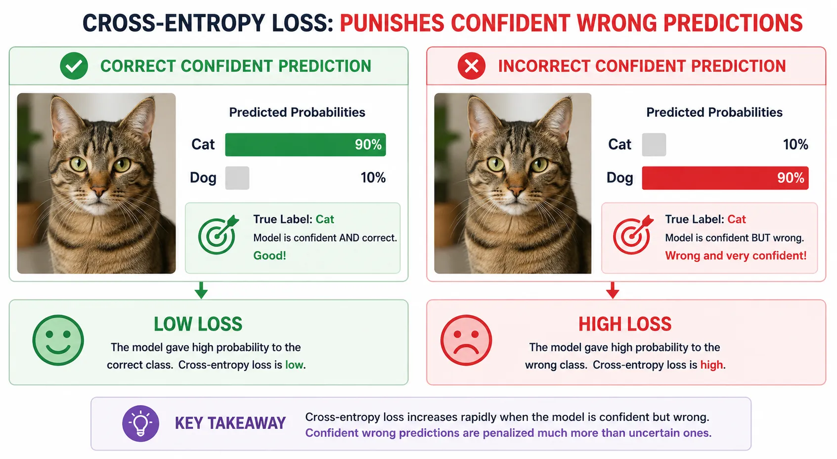
Imagine we are building an image classifier that decides whether a photo contains a cat or a dog.
The real image contains a cat.
Now look at two predictions.
Model A:
Cat: 90%
Dog: 10%
The model gives a high probability to the correct class.
So the cross-entropy loss will be low.
Now consider another prediction.
Model B:
Cat: 10%
Dog: 90%
The real answer is still cat, but this model is highly confident that the image contains a dog.
Cross-entropy gives this prediction a much larger penalty.
That behaviour makes sense.
Being slightly uncertain is one thing.
Being extremely confident about the wrong answer is much worse.
This is one of the main reasons cross-entropy loss is widely used for classification problems.
How Does Cross-Entropy Work?
The full mathematical formula can look intimidating at first, but the idea behind it is surprisingly simple.
For the correct class, cross-entropy roughly asks:
“How much probability did the model give to the correct answer?”
A simplified idea is:
Loss = −log(Probability of the correct class)
You do not need to master logarithms to understand what this means.
Just remember this pattern:
Correct class gets high probability → Low loss
Correct class gets low probability → High loss
For example, imagine the correct answer is “cat.”
If the model gives cat a probability of:
0.95
the loss will be very small.
If the model gives cat:
0.60
the loss becomes larger.
If it gives cat only:
0.05
the loss becomes very large.
So cross-entropy encourages the neural network to become not only correct, but also more confident in the correct classes.
Why Does Cross-Entropy Punish Confident Mistakes?
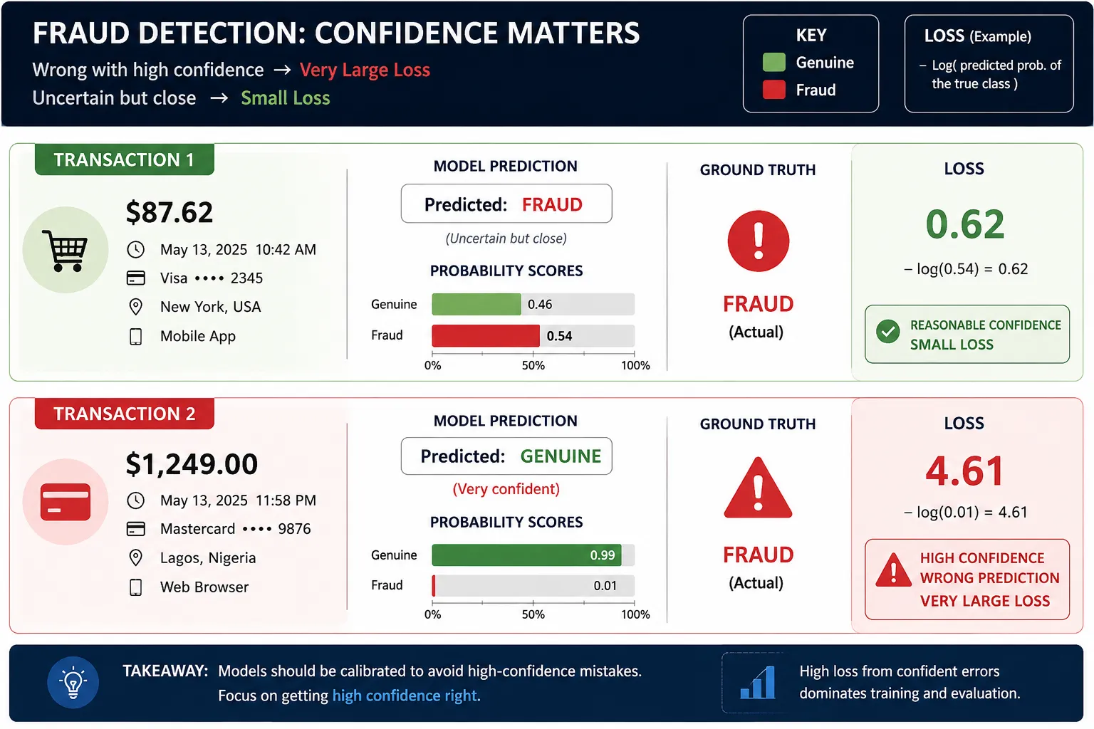
Consider a fraud detection system used by a payment company.
Transaction A is genuine.
The model predicts:
Genuine: 55%
Fraud: 45%
The model is correct, but it is not very confident.
Now suppose Transaction B is actually fraudulent.
The model predicts:
Genuine: 99%
Fraud: 1%
This second mistake is far more serious.
The system did not simply miss the correct answer. It was almost completely confident in the wrong answer.
Cross-entropy is designed to give such predictions a strong penalty.
That stronger training signal tells the neural network:
“Your current decision pattern needs a major correction.”
During backpropagation, this loss helps guide the updates made to the model's weights.
Binary Cross-Entropy: When There Are Two Choices
When a classification problem has two possible outcomes, we commonly use Binary Cross-Entropy, often called BCE.
Examples include:
Spam or not spam
Fraud or genuine
Disease detected or not detected
Customer will leave or stay
Loan default or no default
Positive review or negative review
The true label is usually represented using:
0 or 1
Suppose we are predicting whether a customer will cancel a subscription.
The real answer is:
Customer will cancel = 1
The model predicts:
0.90
That is a strong prediction because it is close to the real target.
Now imagine the model predicts:
0.08
That is far from the correct answer, so binary cross-entropy produces a much larger loss.
In frameworks such as TensorFlow and Keras, Binary Crossentropy is specifically provided for binary 0/1 classification tasks.
Categorical Cross-Entropy: When There Are Multiple Classes
What happens when we have more than two choices?
Imagine a neural network that looks at a photo and chooses between:
Cat
Dog
Horse
Now the model may output:
Cat: 0.70
Dog: 0.20
Horse: 0.10
If the actual image contains a cat, this is a fairly good prediction.
But suppose it outputs:
Cat: 0.02
Dog: 0.03
Horse: 0.95
while the real answer is still cat.
The model has placed almost all of its confidence in the wrong class.
Categorical cross-entropy produces a large loss for that prediction.
This type of loss is commonly used when one example belongs to one class from several possible classes.
Think about tasks such as:
Recognizing handwritten digits from 0 to 9
Classifying an animal species
Identifying the topic of a news article
Recognizing objects in images
Choosing between several product categories
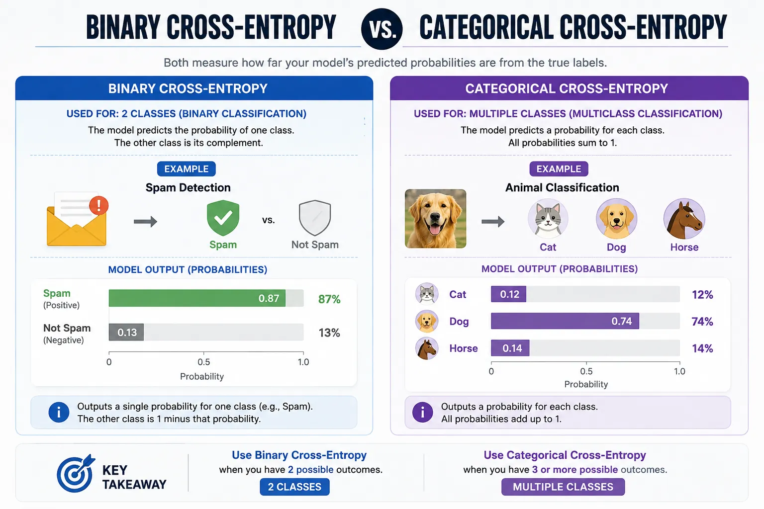
Binary vs Categorical Cross-Entropy
The easiest way to remember the difference is this:
Binary Cross-Entropy → usually two-class decisions
Categorical Cross-Entropy → usually multiple-class decisions
There is also something called Sparse Categorical Cross-Entropy.
It solves the same type of multi-class problem, but the labels are stored differently.
For example, imagine three classes:
Cat = 0
Dog = 1
Horse = 2
With sparse categorical cross-entropy, the correct label can simply be stored as:
Dog = 1
Instead of representing it as something like:
Cat = 0, Dog = 1, Horse = 0
The basic learning idea remains the same. The difference is mainly how the target labels are represented.
Probabilities vs Logits: A Term Beginners Often Meet
While working with TensorFlow, Keras, or PyTorch, you will eventually see the word logits.
It sounds complicated, but the idea is simple.
Before a neural network converts its output into clean probabilities such as:
Cat: 70%
Dog: 20%
Horse: 10%
it usually produces raw scores.
Those raw scores are called logits.
A function such as softmax can convert multi-class logits into probabilities.
For binary classification, sigmoid is commonly used to turn an output into a value between 0 and 1.
Some loss implementations can accept probabilities, while others are designed to work directly with logits. For example, PyTorch's CrossEntropyLoss expects unnormalized logits, and TensorFlow/Keras cross-entropy losses provide a from_logits option.
The important beginner lesson is:
Always check whether your loss function expects logits or probabilities.
Using the wrong format can create incorrect or unstable training behaviour.
MSE vs Cross-Entropy: The Main Difference
Now the bigger picture becomes much easier to see.
Mean Squared Error asks:
“How far is my predicted number from the real number?”
That makes it a natural fit for many regression problems.
Cross-entropy asks something closer to:
“How much probability did I give to the correct class?”
That makes it a natural fit for many classification problems.
Suppose we are building two neural networks.
The first predicts:
Tomorrow's electricity demand = 4,500 MW
That is a number, so a regression loss such as MSE may make sense.
The second predicts:
Payment = Fraud or Genuine
That is a classification problem, so cross-entropy is usually the more natural choice.
This gives us a useful rule:
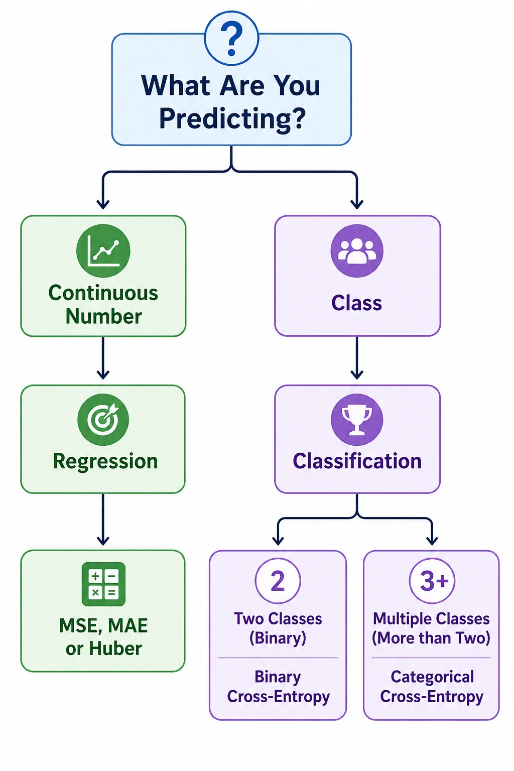
Predicting a continuous number? Think about regression losses such as MSE.
Predicting a class or probability? Think about classification losses such as cross-entropy.
But this rule is only the beginning.
Choosing the right loss function also depends on outliers, class imbalance, model output, label format, and the real cost of making different mistakes.
And that is where choosing between MSE, cross-entropy, and other loss functions becomes much more practical than simply memorizing their formulas.
How to Choose the Right Loss Function
At this point, MSE and cross-entropy may both seem simple enough.
But in a real project, the difficult question is not:
“What does this formula mean?”
The real question is:
“Which loss function should I actually use?”
A good starting point is to look at what your neural network is trying to predict.
If the output is a continuous number such as price, temperature, demand, distance, or delivery time, you are usually dealing with regression.
In that case, Mean Squared Error is often a strong starting choice.
If the output is a category such as spam/not spam, cat/dog, fraud/genuine, or one class out of many possible classes, you are dealing with classification.
In that case, some form of cross-entropy loss will usually make more sense.
But real data is rarely perfect. That is why we need to go one step deeper.
When Should You Use MSE?
MSE works well when your model predicts continuous numerical values and large mistakes should receive a stronger penalty.
Imagine an electricity company trying to predict tomorrow's power demand.
The real demand is:
5,000 MW
Prediction A says:
4,950 MW
The error is small.
Prediction B says:
3,500 MW
That prediction could create a much bigger planning problem.
Because MSE squares errors, Prediction B receives a much stronger penalty.
This is useful when large misses matter.
Common examples include:
House price prediction
Temperature forecasting
Sales forecasting
Energy demand prediction
Travel time estimation
Demand prediction
However, remember the weakness we discussed earlier.
MSE can be strongly affected by unusual values.
If your dataset contains many extreme outliers, blindly choosing MSE may not always be the best option.
What If Your Regression Data Has Outliers?
Imagine a delivery-time dataset where most orders arrive between 20 and 60 minutes.
Then one order takes 600 minutes because the vehicle breaks down.
That single value is very different from normal orders.
Because MSE squares the error, an unusual example like this can have a large effect on training.
One alternative is Mean Absolute Error (MAE).
Instead of squaring the difference, MAE uses the absolute difference between the predicted and actual values.
Another useful option is Huber loss.
Huber loss behaves somewhat like MSE for smaller errors but becomes more like absolute error when mistakes become large.
This can make it less sensitive to extreme errors than pure squared-error loss.
So the lesson is not:
“MSE is always best for regression.”
A better lesson is:
“MSE is a strong starting point, but the shape and quality of your data still matter.”
When Should You Use Cross-Entropy?
Use cross-entropy when your neural network is predicting classes or class probabilities.
For a simple two-class problem such as:
Fraud or genuine
you will commonly see binary cross-entropy.
For a problem with several classes such as:
Car, bike, bus, truck, or train
you will commonly use categorical cross-entropy or sparse categorical cross-entropy, depending on how your labels are stored.
But there is another real-world issue that beginners should understand.
That issue is class imbalance.
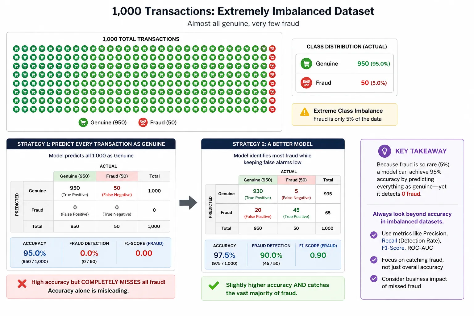
What Happens When the Classes Are Imbalanced?
Imagine building a fraud detection model from one million transactions.
Suppose:
990,000 transactions are genuine.
Only 10,000 are fraudulent.
Now imagine a terrible model that predicts:
“Genuine” for every transaction.
It would still be correct about 99% of the time.
That sounds impressive.
But the model would completely fail at the job we actually care about: detecting fraud.
This is why accuracy alone can be misleading when classes are heavily imbalanced.
The loss function can also be adjusted so mistakes on an important or rare class receive more attention.
For example, classification loss implementations may allow class weights or positive-class weighting.
This can make an error on the rare class more costly during training.
In our fraud example, missing a fraudulent payment may receive more weight than correctly identifying another ordinary genuine transaction.
This does not mean you should randomly increase weights.
The weight should reflect the dataset and the real problem you are solving.
Loss vs Accuracy: They Are Not the Same Thing
This is one of the most important ideas to understand.
Loss and accuracy are not the same measurement.
Imagine two models correctly classify the same image as a dog.
Model A predicts:
Dog: 51%
Cat: 49%
Model B predicts:
Dog: 98%
Cat: 2%
Both models made the correct final decision.
So for this example, their accuracy result is the same.
But their cross-entropy losses are different.
Model B placed much more probability on the correct answer, so it receives a lower loss.
Now suppose another model predicts:
Dog: 1%
Cat: 99%
when the real image contains a dog.
That highly confident wrong prediction receives a much larger loss.
This is why you might sometimes see training logs where accuracy barely changes while loss continues falling.
The model may not be changing many final class decisions yet, but it may be becoming more confident in correct predictions.
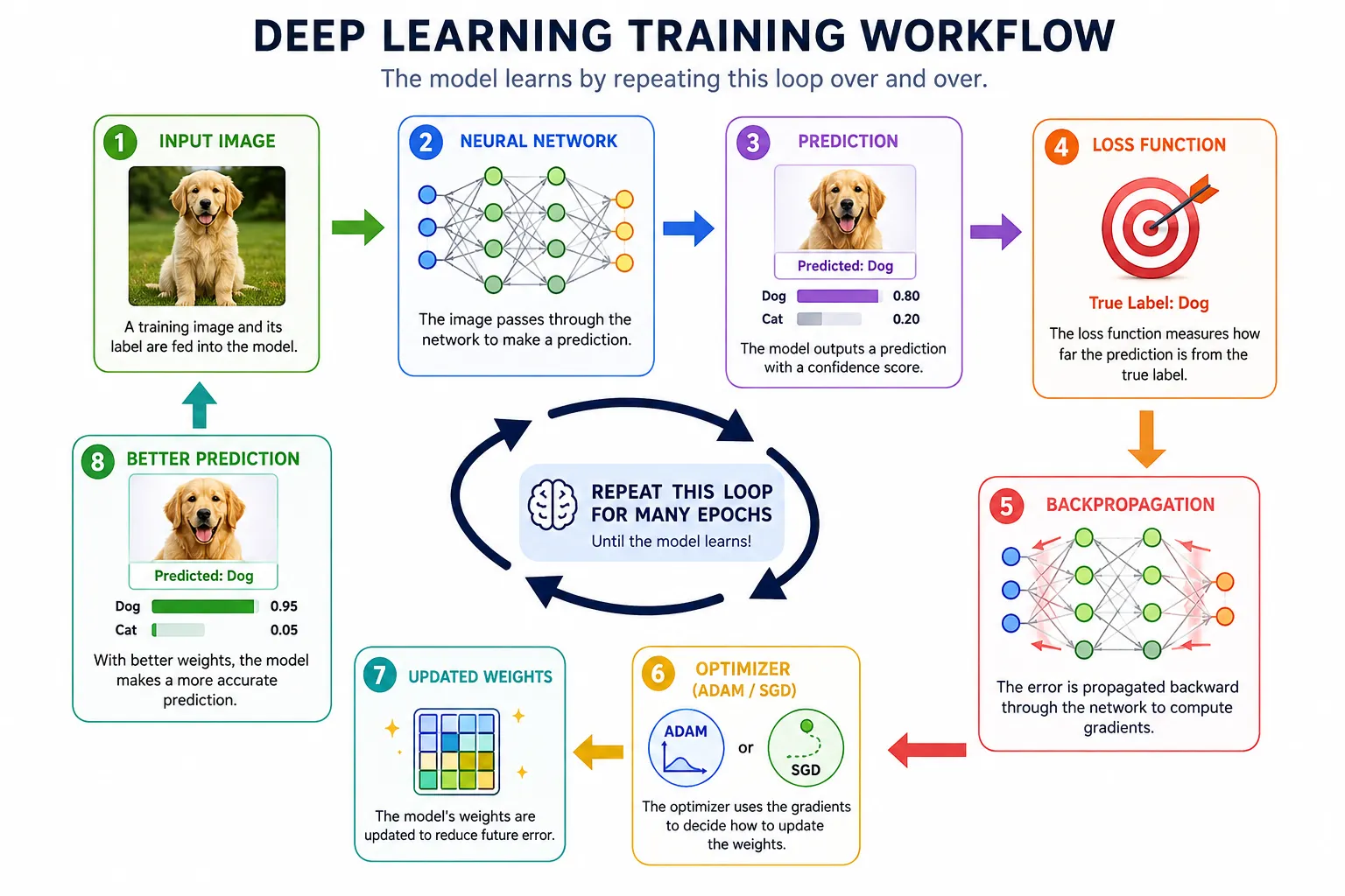
How Loss Helps a Neural Network Learn
Now we can connect everything together.
Imagine a neural network sees an image of a cat.
Step 1: The Network Makes a Prediction
It predicts:
Cat: 30%
Dog: 70%
The answer is wrong.
Step 2: The Loss Function Measures the Mistake
Cross-entropy looks at the low probability given to the correct class and produces a relatively high loss.
Step 3: Backpropagation Finds What Should Change
The network calculates how its internal weights contributed to that loss.
Step 4: The Optimizer Updates the Weights
An optimizer such as SGD or Adam changes the weights in a direction intended to reduce the loss.
Step 5: The Network Tries Again
After many training examples and repeated updates, the model hopefully begins producing better predictions.
The full idea is:
Prediction → Loss → Backpropagation → Optimizer → Weight Update → Better Prediction
This is why the loss function is so important.
It gives the training process a target to improve.
Without a meaningful loss function, the optimizer would not have a useful objective telling it which direction represents improvement.
Common Loss Function Mistakes Beginners Make
One common mistake is using MSE for every problem simply because its formula is easy to understand.
MSE is excellent for many regression tasks, but classification usually has better-suited losses such as cross-entropy.
Another mistake is choosing binary cross-entropy when the label structure actually represents a different type of multi-class problem.
A third mistake is ignoring whether the model outputs logits or probabilities.
Your neural network output and your loss function must be configured correctly together.
Another common problem is focusing only on the training loss.
If training loss keeps falling while validation performance gets worse, the model may be overfitting instead of genuinely learning patterns that work on new data.
Finally, never judge a model using only one number.
Loss helps train the neural network, but real evaluation may also require metrics such as accuracy, precision, recall, F1-score, or other task-specific measurements.
MSE vs Cross-Entropy: The Rule Worth Remembering
You do not need to memorize every loss function before building your first neural network.
Start with the problem.
Ask:
What am I predicting?
If the answer is a continuous numerical value, start by thinking about regression losses such as MSE.
If the answer is a class, start by thinking about cross-entropy loss.
Then look deeper.
Are there outliers?
Are the classes imbalanced?
Does the model output logits or probabilities?
What kinds of mistakes are most expensive in the real world?
Those questions matter more than memorizing formulas.
A loss function may look like one small line of mathematics inside your code, but it defines what the neural network considers a mistake.
And once you understand that idea, MSE and cross-entropy stop looking like difficult formulas.
They become something much simpler:
Different ways of teaching a neural network what it needs to improve.
Frequently Asked Questions About Loss Functions
What Is a Loss Function?
A loss function measures how far a model's prediction is from the correct answer. During training, the neural network tries to reduce this loss so its future predictions become more accurate.
Why Do Neural Networks Need Loss Functions?
A neural network needs a loss function to understand how good or bad its predictions are. The loss gives the training process a clear target and helps backpropagation and the optimizer decide how the model's weights should change.
How Does MSE Work?
Mean Squared Error calculates the difference between predicted and actual values, squares each difference, and then finds their average. Smaller MSE usually means the regression model's predictions are closer to the real values.
Why Is Error Squared in MSE?
Squaring prevents positive and negative errors from cancelling each other out. It also gives larger mistakes a much stronger penalty, which encourages the model to pay more attention to large prediction errors.
When Should I Use Cross-Entropy Loss?
Cross-entropy is usually used for classification problems. Binary cross-entropy works well for two-class problems, while categorical or sparse categorical cross-entropy is commonly used when a model must choose between several classes.
Can MSE Be Used for Classification?
Technically, MSE can be used in some classification setups, but it is usually not the best choice. Cross-entropy is generally better suited because it directly works with class probabilities and strongly penalizes confident wrong predictions.
What Is the Difference Between Loss and Accuracy?
Accuracy tells you how many final predictions were correct. Loss measures how good or bad those predictions were, including model confidence. Two models can have the same accuracy while having very different loss values.


