


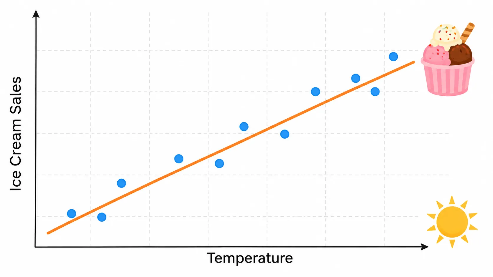
Imagine you run a small ice cream shop.
On cool days, you sell around 70 cups. On very hot days, you may sell more than 200. After watching this pattern for a few months, you wonder:
“Can tomorrow’s temperature help me estimate how many ice creams to prepare?”
That is the kind of problem linear regression helps solve.
It studies how a numeric outcome changes when one or more input values change. Here, temperature is the input, and ice creams sold is the outcome.
Instead of guessing, linear regression uses past data to find a trend and make a reasonable prediction.
What Is Linear Regression in Simple Words?
Linear regression is a statistical and machine learning method used to understand a relationship and predict a number.
It looks for a general pattern in known data and represents that pattern using a line or a linear equation.
Think of it as placing a ruler through a cloud of dots.
The dots are real observations. The ruler is the model.
The ruler may not touch every dot because real-world data is rarely perfect. However, it should capture the overall direction of the data.
Once the line has been found, we can use it to estimate an unknown value.
For example, linear regression can help us:
Predict a house price from its floor area
Estimate delivery time from travel distance
Predict monthly sales from advertising spend
Estimate electricity use from temperature
Predict an exam score from study hours
Simple linear regression studies the relationship between one numeric predictor and one numeric response. These are commonly called the independent variable and dependent variable.
The final output is normally a number.
For example:
₹45,000 monthly sales
72 exam marks
35 minutes of delivery time
₹60 lakh house price
When the goal is to predict a category such as “spam or not spam,” “approved or rejected,” or “cat or dog,” the problem is classification, not ordinary linear regression.
Why Beginners Should Learn Linear Regression First
Linear regression teaches several important machine learning ideas through one understandable model.
It introduces:
Features and targets
Training data
Model predictions
Prediction errors
Model coefficients
Loss functions
Model evaluation
You will meet these same ideas again when studying decision trees, neural networks, support vector machines and other machine learning algorithms.
Linear regression is also easy to inspect.
You can usually understand why a prediction increased or decreased instead of treating the model like a complete black box.
This makes linear regression valuable not only for learning but also for forecasting, scientific research, business analysis and baseline machine learning models.
A baseline model gives you a simple result to compare against. It helps you judge whether a more complex model is actually providing better predictions.
The Core Mental Model: Find the Best Trend
Suppose five students study for different numbers of hours.
Study Hours
Exam Score
1
48
2
55
3
63
4
72
5
78
The exam score does not increase by exactly the same amount after every additional study hour.
However, the direction is clear.
As study time increases, the score generally increases too.
Linear regression tries to capture this direction using one line.
The line helps answer a useful question:
“Based on the available data, what score would we expect for a given number of study hours?”
For example, we could use the pattern to estimate the score of a student who studies for six hours.
However, the prediction will not be a guarantee.
Sleep, stress, prior knowledge, teaching quality and exam difficulty may also affect the result. Our model only summarizes the relationship represented by the data we provide.
This gives us one of the most important lessons in machine learning:
A prediction is an informed estimate, not a promise.
Understanding the Linear Regression Equation
A simple linear regression model is commonly written as:
[
\hat{y} = b_0 + b_1x
]
You may also see the complete form:
[
y = b_0 + b_1x + \epsilon
]
The symbols may look technical, but each one has a simple role.
Symbol
Meaning
(x)
Input or predictor
(y)
Actual outcome
(\hat{y})
Predicted outcome
(b_0)
Intercept
(b_1)
Slope or coefficient
(\epsilon)
Unexplained error
For multiple features, the same idea is extended by giving each input its own coefficient or weight.
What Does the Slope Mean?
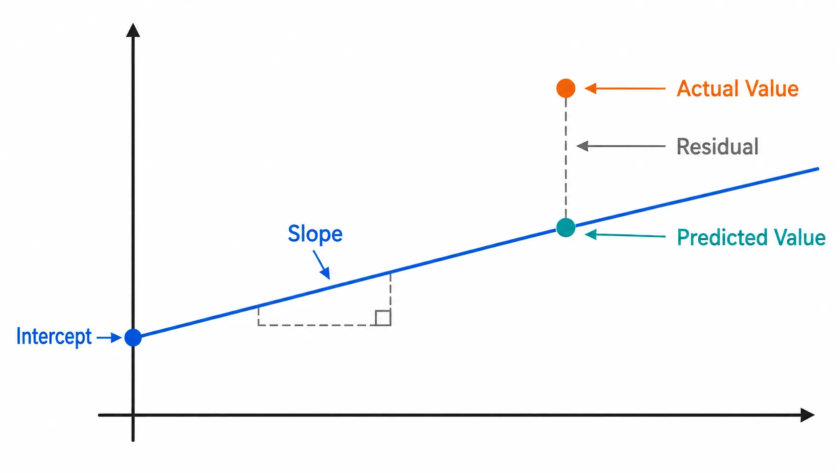
The slope tells us how much the predicted outcome changes when the input increases by one unit.
Suppose our student-score model is:
[
\text{Predicted Score} = 40 + 8 \times \text{Study Hours}
]
The slope is 8.
This means the model predicts an average increase of 8 marks for every additional study hour.
For three hours of study:
[
40 + 8(3) = 64
]
The predicted exam score is 64.
A positive slope rises from left to right.
It suggests that the predicted outcome increases when the input increases.
A negative slope falls from left to right.
For example, a model studying product price and customer demand may learn a negative slope. As the price increases, the expected demand may decrease.
What Does the Intercept Mean?
The intercept is the predicted value when the input is zero.
In our exam-score equation, the intercept is 40.
The model predicts a score of 40 when study time is zero.
However, the intercept is not always meaningful in the real world.
Suppose you create a model that predicts crop growth using temperature. An input temperature of zero degrees may be outside the useful range of the data you collected.
In such cases, the intercept is still needed for the equation, but its real-world interpretation may not be useful.
A good rule is:
Treat the intercept as part of the mathematical model first. Interpret it only when an input value of zero makes sense.
Independent and Dependent Variables
Beginners often mix up independent and dependent variables.
The independent variable is the input used to explain or predict something.
It may also be called:
Feature
Predictor
Explanatory variable
Input variable
The dependent variable is the numeric result that we want to predict.
It may also be called:
Target
Response
Label
Outcome
Output variable
In our ice cream example:
Temperature is the independent variable
Number of ice creams sold is the dependent variable
A simple memory trick is:
The predicted result depends on the input.
However, the term “independent variable” does not mean that the variable definitely causes the outcome.
Regression can show that two variables are associated. It does not automatically prove that changing one variable will cause the other variable to change.
Simple vs Multiple Linear Regression
Linear regression has two common forms.
Simple Linear Regression
Simple linear regression uses one predictor.
[
\text{Sales} = b_0 + b_1(\text{Advertising Spend})
]
Here, advertising spend is the only input used to predict sales.
Multiple Linear Regression
Multiple linear regression uses two or more predictors.
[
\text{Sales} =
b_0 +
b_1(\text{Advertising Spend}) +
b_2(\text{Product Price}) +
b_3(\text{Season})
]
The basic idea remains the same.
Each feature receives a coefficient that represents its contribution to the prediction while the other included features are held constant.
Real-world outcomes usually depend on several factors.
A house price may depend on:
Floor area
Location
Property age
Number of rooms
Parking availability
Nearby schools and hospitals
Multiple linear regression can represent more of this reality.
However, adding more features does not automatically produce a better model. Irrelevant or highly related features may make the model harder to understand and less reliable.
How Does Linear Regression Choose the Best Line?
Many different lines can pass through the same group of data points.
Linear regression needs a rule for deciding which line is best.
For every observation, the model compares the actual value with its predicted value:
[
\text{Residual} =
\text{Actual Value} -
\text{Predicted Value}
]
This difference is called a residual or prediction error.
A small residual means the prediction is close to the real value.
A large residual means the model made a larger mistake.
A common method called ordinary least squares chooses the line that minimizes the sum of the squared residuals. Scikit-learn’s LinearRegression estimator uses this residual-sum-of-squares objective, while Google describes loss as a numerical measurement of how wrong a model’s predictions are.
Why do we square the errors?
First, squaring stops positive and negative errors from cancelling each other.
Second, it penalizes larger mistakes more strongly.
This is the mathematical engine behind the best-fit line.
How Linear Regression Learns from Its Mistakes
we learned that linear regression finds a straight line that represents the general pattern in our data.
But an important question is still unanswered:
How does the model know whether one line is better than another?
To understand that, imagine you are throwing a basketball toward a hoop.
Your first shot falls short. The next shot goes too far. After each attempt, you notice the mistake and adjust your next shot.
Linear regression works in a similar way.
It compares its predictions with the actual answers, measures how wrong it was, and finds the line that produces the smallest overall error.
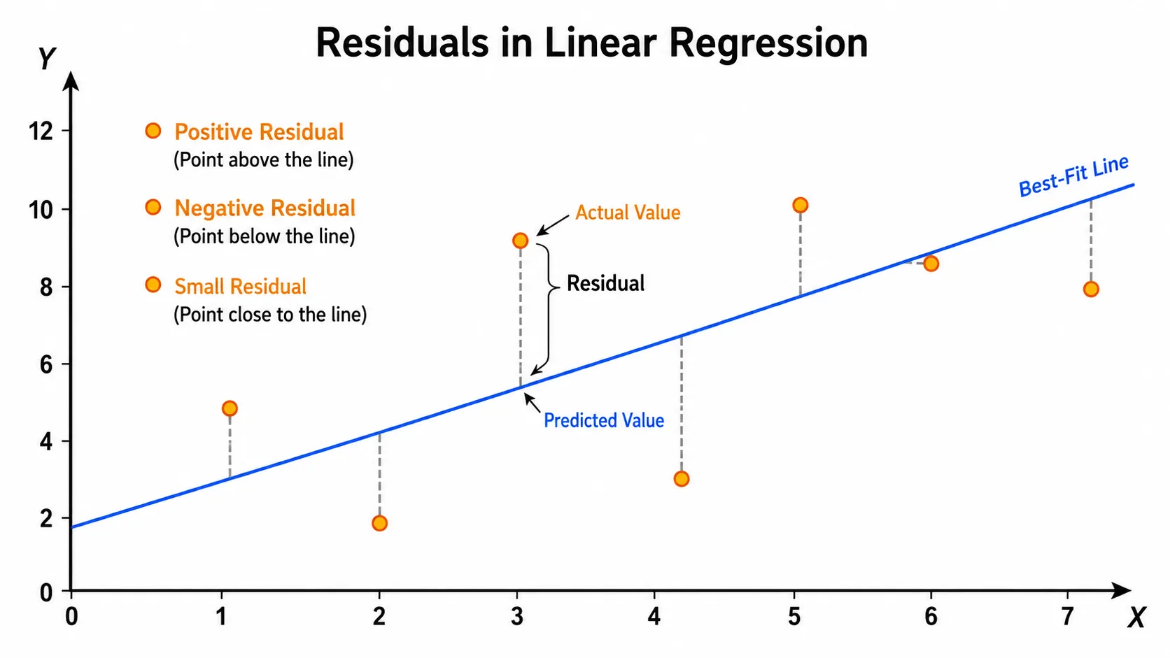
This difference between prediction and reality is called a residual.
What Is a Residual?
A residual is the difference between the actual value and the value predicted by the regression model.
The formula is:
[
\text{Residual} = \text{Actual Value} - \text{Predicted Value}
]
Suppose a model predicts that a student will score 70 marks, but the student actually scores 76.
The residual is:
[
76 - 70 = 6
]
The model underestimated the score by 6 marks.
Now suppose the model predicts 82 marks, but the actual score is 76.
The residual becomes:
[
76 - 82 = -6
]
The negative sign means that the model predicted a value higher than the actual result.
Residuals help us understand the direction and size of each prediction mistake.
A residual close to zero means the prediction was close to the actual value.
A large positive or negative residual means the prediction was far from reality.
Why Can We Not Simply Add All Errors?
Suppose a model makes the following two mistakes:
It underestimates one value by 10
It overestimates another value by 10
If we add these errors directly, we get:
[
10 + (-10) = 0
]
This result makes the model look perfect, even though it made two clear mistakes.
That is why linear regression does not simply add raw residuals.
Instead, it squares every residual before adding them.
[
\text{Squared Error} = (\text{Actual} - \text{Predicted})^2
]
When a residual is squared, both positive and negative values become positive.
For example:
[
10^2 = 100
]
[
(-10)^2 = 100
]
Now the two errors cannot cancel each other.
Their total squared error becomes:
[
100 + 100 = 200
]
This gives us a more honest measurement of how wrong the model is.
What Is the Least Squares Method?
The least squares method is the process used to find the line with the smallest total squared error.
Imagine placing many possible lines through the same group of data points.
One line may be too high.
Another may be too low.
Another may fit some points well but miss several others badly.
For every possible line, we can calculate the squared residuals and add them together.
The line with the lowest total is selected as the best-fit line.
This total is called the sum of squared errors.
[
SSE = \sum (y - \hat{y})^2
]
The symbol (\sum) simply means that we calculate the squared error for every data point and then add all the results.
The model is not trying to pass through every single point.
It is trying to find a balanced line that performs well across the complete dataset.
Think of it like drawing a road through several villages.
The road may not pass directly through every house, but it should follow a route that keeps the total travelling distance as small as possible.
Understanding Loss Functions
A loss function tells us how bad a model’s predictions are.
It converts prediction mistakes into a single number.
A lower loss usually means that the model is making better predictions.
A higher loss means that the predictions are further away from the actual values.
During model training, the goal is to reduce this loss.
Different regression problems may use different loss functions. However, squared error is one of the most common choices because it gives more importance to large mistakes.
For example, compare these two residuals:
[
2^2 = 4
]
[
10^2 = 100
]
The second error is five times larger before squaring, but its squared penalty is twenty-five times larger.
This means squared error strongly punishes predictions that are far from reality.
That can be useful when large mistakes are especially costly.
For example, predicting a delivery five minutes late may be acceptable. Predicting it two hours late may create a serious customer experience problem.
Training Error and Test Error
A model should not only perform well on the data it has already seen.
It should also work well on new data.
That is why a dataset is normally divided into two parts:
Training data
Test data
The model learns the regression line from the training data.
The test data is kept separate and used later to measure how well the model performs on unseen examples.
Imagine a student who memorizes all the answers from a practice paper.
The student may score perfectly on the same paper but struggle when the questions change.
A machine learning model can face the same problem.
When a model learns the training data too closely, including its random noise, it is called overfitting.
An overfitted model performs well on training data but poorly on new data.
On the other hand, a model that is too simple to capture the real pattern is called underfitted.
An underfitted model performs poorly on both training and test data.
The goal is to find a balance where the model learns the real pattern without memorizing every small irregularity.
Mean Absolute Error
Mean Absolute Error, commonly called MAE, measures the average size of prediction errors.
It ignores whether an error is positive or negative.
[
MAE = \frac{1}{n}\sum |y - \hat{y}|
]
The vertical bars mean that we take the absolute value of every residual.
Suppose the prediction errors are:
3
-5
4
Their absolute values are:
3
5
4
The MAE is:
[
\frac{3 + 5 + 4}{3} = 4
]
This means the model is wrong by about 4 units on average.
MAE is easy to explain because it uses the same unit as the target.
If we are predicting house prices in lakhs, the MAE is also measured in lakhs.
Mean Squared Error
Mean Squared Error, or MSE, calculates the average of squared prediction errors.
[
MSE = \frac{1}{n}\sum (y - \hat{y})^2
]
Because errors are squared, large mistakes receive a much heavier penalty.
This makes MSE useful when major prediction errors are more dangerous than small ones.
However, its unit is also squared.
If the target is measured in rupees, MSE is measured in squared rupees, which is harder to explain to a non-technical reader.
Root Mean Squared Error
Root Mean Squared Error, or RMSE, solves the unit problem of MSE.
It calculates the square root of the mean squared error.
[
RMSE = \sqrt{MSE}
]
RMSE returns the error to the original unit of the target.
Like MSE, it gives more importance to large mistakes.
Suppose a house-price model has an RMSE of ₹4 lakh.
This means its predictions are typically around ₹4 lakh away from actual prices, although the exact interpretation depends on the distribution of errors.
MAE and RMSE are often compared together.
When RMSE is much larger than MAE, it can be a sign that the model is making a few very large mistakes.
Understanding R-Squared
Another common evaluation metric is R-squared, written as:
[
R^2
]
R-squared measures how much of the variation in the target is explained by the model.
Its value is often between 0 and 1.
An (R^2) of 0 means that the model does not explain the variation better than simply predicting the average value.
An (R^2) of 1 means that the model perfectly explains all observed variation in the dataset.
Suppose a house-price model has an (R^2) of 0.80.
A simple interpretation is that the model explains around 80% of the variation in house prices represented by the data.
However, a high R-squared does not automatically mean that the model is useful.
The model may still:
Make large prediction errors
Perform poorly on new data
Use irrelevant features
Miss a non-linear pattern
Be affected by outliers
That is why R-squared should not be used alone.
It is better to examine it together with MAE, RMSE, residuals and test-set performance.
Important Assumptions of Linear Regression
Linear regression works best when some basic conditions are reasonably satisfied.
First, the relationship between inputs and the target should be approximately linear.
If the data follows a strong curve, a straight line may not represent it properly.
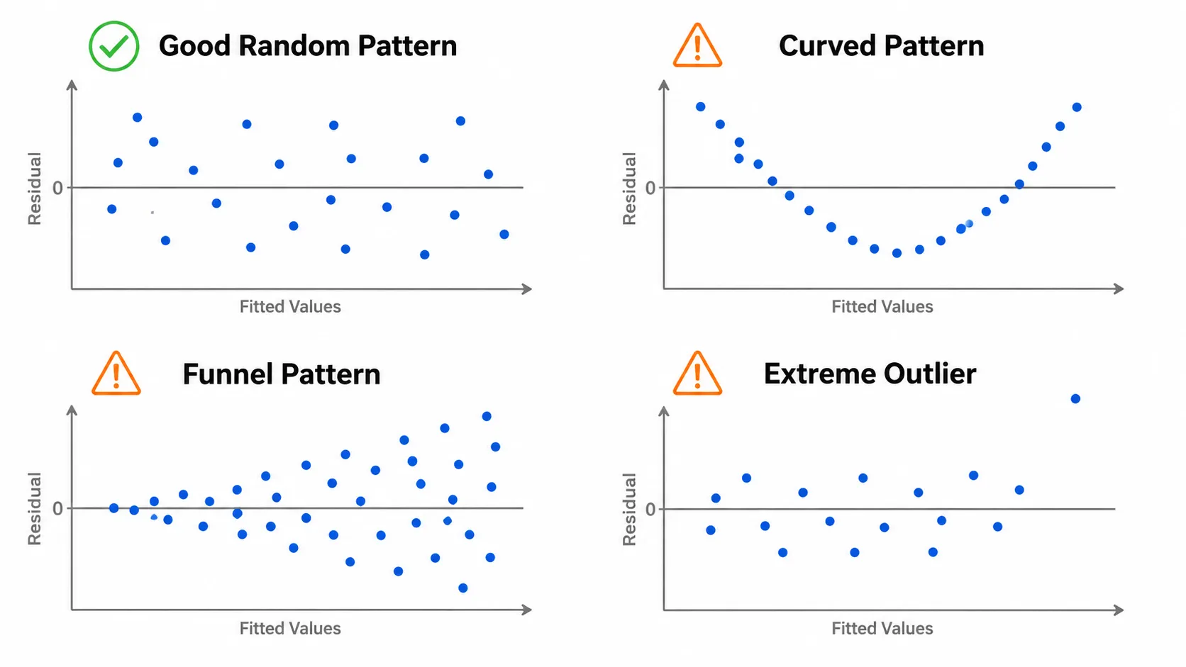
Second, residuals should not show a clear pattern.
If residuals form a curve, wave or funnel shape, the model may be missing important information.
Third, observations should be reasonably independent.
For example, today’s sales may be connected to yesterday’s sales. Time-based data may require special handling.
Fourth, extreme outliers should be investigated.
One unusual point can pull the regression line strongly in one direction.
Finally, in multiple linear regression, input variables should not be almost identical to each other.
For example, using both a person’s age in years and age in months provides nearly the same information. This can make model coefficients unstable.
These assumptions do not mean that real data must be perfect.
They help us identify when linear regression is a sensible choice and when another approach may work better.
The Main Idea to Remember
Linear regression learns by measuring the distance between its predictions and the real answers.
It squares those distances, adds them together and chooses the line with the lowest total error.
After training, we evaluate the model on unseen data using measures such as MAE, MSE, RMSE and R-squared.
The most important lesson is simple:
A good regression model is not the line that memorizes every point. It is the line that captures the real pattern and continues to make useful predictions on new data.
Building a Linear Regression Model in Python
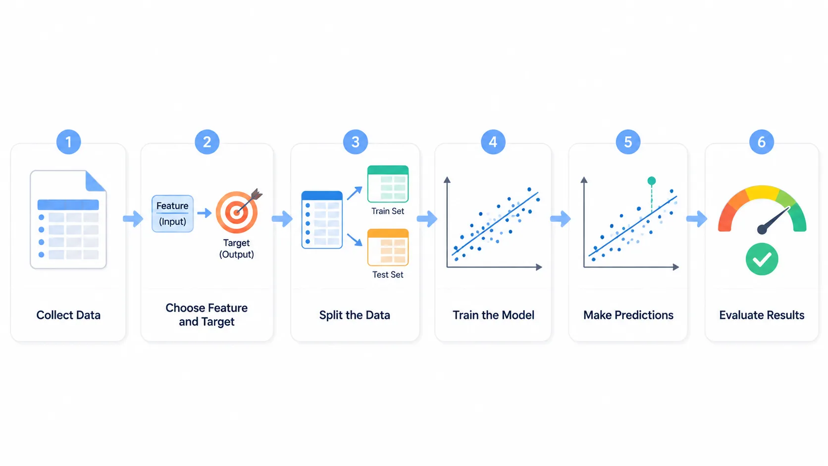
So far, we have understood what linear regression does, how it finds the best-fit line and how we measure its mistakes.
Now let us turn that knowledge into a working Python model.
We will use a simple example:
Can we predict a student’s exam score from the number of hours they study?
Our dataset will be small so that every step remains easy to understand.
Installing the Required Libraries
We will use three popular Python libraries:
NumPy for storing numeric data
Matplotlib for creating graphs
Scikit-learn for building and evaluating the model
You can install them using:
pip install numpy matplotlib scikit-learn
Once the libraries are installed, we can create our dataset.
Creating a Simple Dataset
import numpy as np
# Number of hours studied
study_hours = np.array([1, 2, 3, 4, 5, 6, 7, 8, 9, 10])
# Exam scores achieved
exam_scores = np.array([45, 50, 56, 63, 67, 74, 78, 84, 88, 94])
Each position in study_hours is connected to the same position in exam_scores.
For example:
A student who studied for 1 hour scored 45
A student who studied for 5 hours scored 67
A student who studied for 10 hours scored 94
Scikit-learn expects the input features to be arranged in rows and columns.
Since we currently have a one-dimensional array, we need to reshape it.
X = study_hours.reshape(-1, 1)
y = exam_scores
X represents the input feature.
y represents the target that we want to predict.
The -1 tells NumPy to calculate the required number of rows automatically. The value 1 means that our dataset contains one input feature: study hours.
Splitting Training and Test Data
We should not train and evaluate the model using exactly the same observations.
Instead, we divide the data into a training set and a test set.
from sklearn.model_selection import train_test_split
X_train, X_test, y_train, y_test = train_test_split(
X,
y,
test_size=0.2,
random_state=42
)
Here, test_size=0.2 means that 20% of the data will be reserved for testing.
The remaining 80% will be used for training.
random_state=42 ensures that the data is split in the same way every time we run the code. The number 42 has no special mathematical meaning. Any fixed integer can be used.
Training the Linear Regression Model
Now we can create and train the model.
from sklearn.linear_model import LinearRegression
model = LinearRegression()
model.fit(X_train, y_train)
The LinearRegression() line creates an empty regression model.
The fit() method allows the model to study the training data.
During this step, the model calculates the slope and intercept that produce the best-fit line.
Checking the Slope and Intercept
print("Slope:", model.coef_[0])
print("Intercept:", model.intercept_)
The slope tells us how much the predicted exam score changes when study time increases by one hour.
Suppose the slope is approximately 5.4.
This means the model predicts that each additional study hour is associated with an average increase of around 5.4 marks.
The intercept represents the predicted score when study time is zero.
Remember that this interpretation is useful only when zero is a sensible input value.
Making a New Prediction
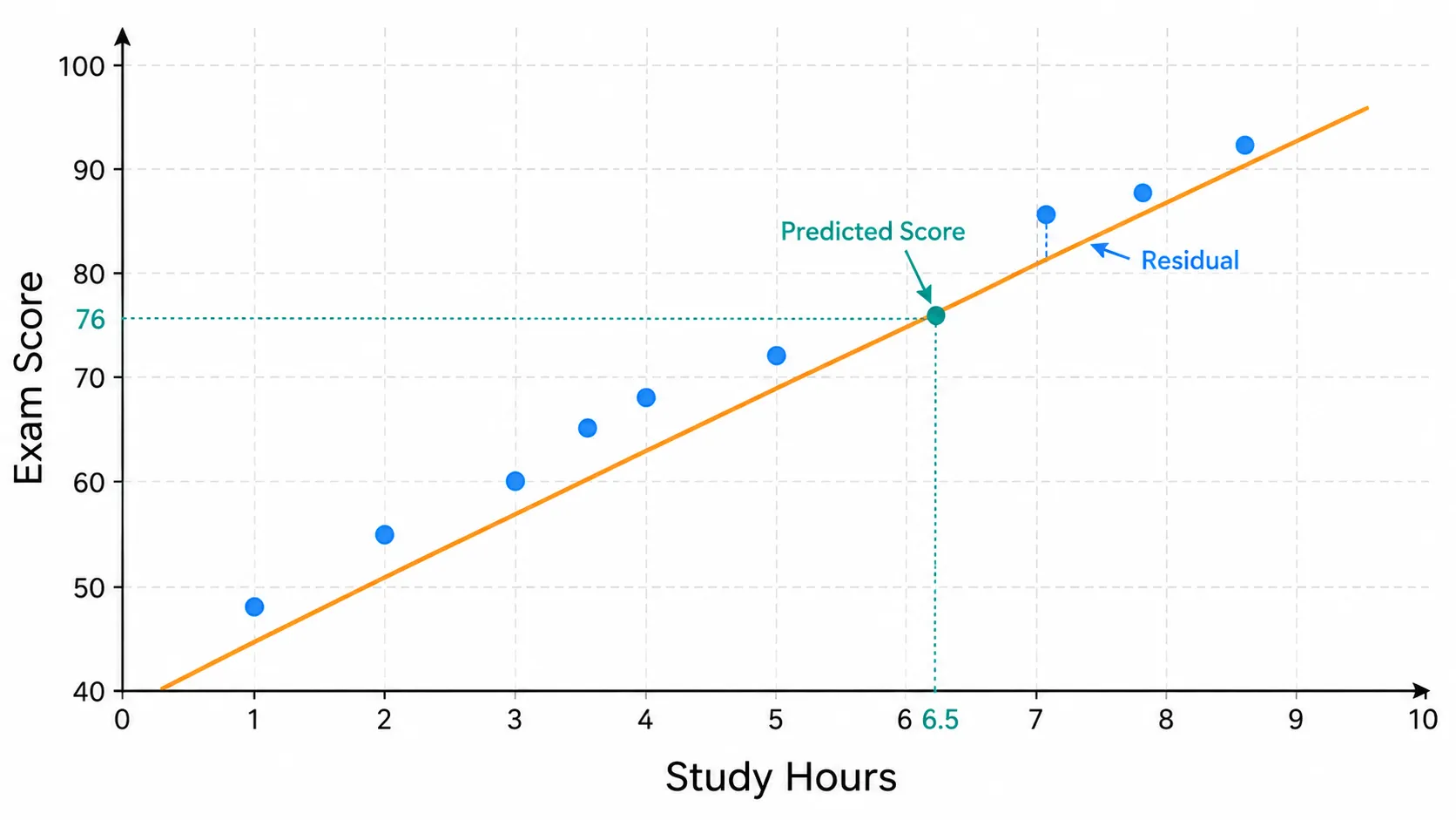
Suppose a student studies for 6.5 hours.
We can estimate the student’s exam score using:
new_student = np.array([[6.5]])
predicted_score = model.predict(new_student)
print("Predicted score:", predicted_score[0])
The input contains two square brackets because scikit-learn expects the data in a two-dimensional format.
The prediction may be around 76 or 77 marks, depending on the exact training split.
This number is an estimate based on the pattern in the available data.
It does not mean that every student who studies for 6.5 hours will receive the same score.
Testing the Model
We can now make predictions for the test data.
y_pred = model.predict(X_test)
print("Actual scores:", y_test)
print("Predicted scores:", y_pred)
Comparing actual and predicted values gives us a basic understanding of model performance.
However, checking values manually is not enough. We should calculate evaluation metrics.
from sklearn.metrics import mean_absolute_error
from sklearn.metrics import mean_squared_error
from sklearn.metrics import r2_score
mae = mean_absolute_error(y_test, y_pred)
mse = mean_squared_error(y_test, y_pred)
rmse = np.sqrt(mse)
r2 = r2_score(y_test, y_pred)
print("MAE:", mae)
print("MSE:", mse)
print("RMSE:", rmse)
print("R-squared:", r2)
MAE tells us the average absolute prediction error.
RMSE also measures prediction error, but it gives a larger penalty to major mistakes.
R-squared shows how much variation in the exam scores is explained by the model.
Because our dataset is extremely small, these results should be treated as a learning example rather than strong evidence about real student performance.
Visualizing the Best-Fit Line
A graph makes linear regression much easier to understand.
import matplotlib.pyplot as plt
plt.scatter(study_hours, exam_scores, label="Actual scores")
predicted_all_scores = model.predict(X)
plt.plot(study_hours, predicted_all_scores, label="Regression line")
plt.xlabel("Study Hours")
plt.ylabel("Exam Score")
plt.title("Study Hours vs Exam Score")
plt.legend()
plt.show()
The dots represent actual observations.
The straight line represents the scores predicted by the model.
Points close to the line have small residuals. Points far from the line have larger residuals.
Common Linear Regression Mistakes
Assuming Correlation Means Causation
A relationship between two variables does not automatically prove that one causes the other.
For example, ice cream sales and electricity usage may both increase during summer. That does not mean buying ice cream directly causes higher electricity usage.
Temperature may be affecting both.
Ignoring Outliers
An unusual data point can pull the regression line in the wrong direction.
Before removing an outlier, investigate it.
It may represent:
A data-entry error
A measurement problem
A rare but real event
An important business case
Do not delete unusual observations simply because they make the model look worse.
Predicting Too Far Outside the Data
Suppose the model was trained using study times between 1 and 10 hours.
Predicting the result for 11 hours may be reasonable.
Predicting the result for 100 hours is not.
Using a model outside the range of its training data is called extrapolation. Such predictions can become unrealistic because the learned relationship may not continue forever.
Using Linear Regression for a Curved Relationship
Some relationships are not straight.
For example, productivity may improve as working hours increase, but after a point, exhaustion may reduce performance.
A straight regression line may miss this curve.
Always inspect the data visually before trusting the model.
Judging the Model Only by R-Squared
A high R-squared does not guarantee accurate or useful predictions.
Check test performance, residual patterns, MAE, RMSE, outliers and the business meaning of the result.
A model should not only look good mathematically. It should solve the actual problem.
Where Is Linear Regression Used?
Linear regression is used in many practical situations.
Businesses use it to estimate sales, demand, costs and advertising results.
Real-estate platforms use regression models to estimate property prices from size, location, age and available facilities.
Hospitals and researchers may use it to study how numeric health outcomes are associated with age, weight, treatment dosage or test results.
Operations teams use it to estimate delivery times, fuel consumption and future resource requirements.
It is also commonly used as a baseline model.
Before building a complex machine learning system, data scientists often train a linear regression model first. If a complicated model cannot clearly outperform the simple baseline, the extra complexity may not be justified.
You will meet these same ideas again when studying decision trees, neural networks, support vector machines and other machine learning algorithms.
Final Takeaway
Linear regression is not just a formula for drawing a straight line.
It is a complete way of thinking about prediction.
You begin with past observations, identify input and target variables, find the best-fit relationship, measure prediction errors and test whether the pattern works on unseen data.
The model is powerful because it is simple, fast and easy to explain.
But its simplicity also creates limits.
It works best when the relationship is reasonably linear, the data is reliable and the predictions remain close to the range represented in the training data.
Remember the ice cream shop from the beginning?
The shop owner does not need to guess tomorrow’s demand blindly. By studying how past sales changed with temperature, linear regression can provide a useful estimate.
It will not predict the future perfectly.
Rain, holidays, local events and customer preferences may still affect sales.
But it transforms a rough feeling—
“Hot days seem busier”
—into a measurable relationship that can be tested, explained and used for better decisions.
That is the real value of linear regression.
It turns past data into a simple line, and that line into a practical prediction.


