


The first time I used logistic regression, I thought the difficult part would be writing the code. It was not. The model took only a few lines to train, returned an accuracy score that looked respectable, and produced predictions without throwing a single error. On paper, everything seemed fine.
Then I checked the individual predictions.
A customer with a 49% predicted chance of leaving was marked as “will stay,” while another customer with a 51% chance was marked as “will leave.” The model appeared confident because the final output showed only 0 and 1, but the actual difference between those two customers was tiny.
I had treated logistic regression like a machine that gives fixed answers. In reality, it was estimating probabilities, and my chosen threshold was converting those probabilities into decisions.
That small misunderstanding changed the way I looked at classification models.
Logistic regression is simple enough to appear in almost every beginner machine learning course, but it is also deep enough to introduce some of the most important ideas in data science: probability, odds, decision boundaries, loss functions, regularization, feature influence, and the trade-off between different kinds of prediction errors.

What Is Logistic Regression?
Logistic regression is a supervised machine learning algorithm commonly used to estimate the probability of a categorical outcome.
In its most familiar form, binary logistic regression answers questions that have two possible outcomes:
Will a customer cancel a subscription?
Is this transaction fraudulent?
Will a visitor click the Buy Now button?
Is an email spam or not spam?
Does a patient show signs of a particular medical condition?
Despite the word “regression” in its name, logistic regression is generally used as a classification algorithm.
However, the model does not begin by directly predicting “yes” or “no.” It first calculates a probability between 0 and 1. A classification threshold is then applied to convert that probability into a final class.
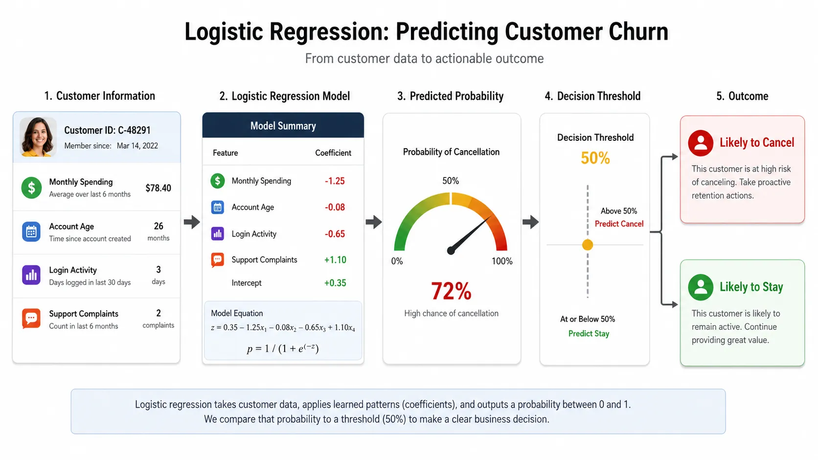
Suppose a model predicts that a customer has a 72% probability of cancelling a subscription. If the classification threshold is 0.5, the customer will be assigned to class 1, which might represent “likely to cancel.”
Another customer with a predicted probability of 0.31 will be assigned to class 0, representing “likely to stay.”
The process can be understood as:
Input data → Predicted probability → Classification threshold → Final class
This distinction is extremely important.
A probability of 0.51 and a probability of 0.95 may produce the same final class, but they do not indicate the same level of confidence. One prediction is only slightly above the decision boundary, while the other is much stronger.
Logistic regression should therefore not be understood as a model that simply predicts zero or one. It is better understood as a model that estimates the probability of an event, after which a separate decision rule converts that probability into a class.
Why Is It Called Regression If It Performs Classification?
This name confuses almost everyone at first.
Logistic regression is used for classification, but the model performs a regression-like operation on the log-odds of the target outcome.
It starts by creating a linear combination of the input features:
z = b₀ + b₁x₁ + b₂x₂ + … + bₙxₙ
In this equation:
The x values represent input features.
The b values represent coefficients learned during training.
b₀ represents the intercept or bias.
z represents the model’s raw linear output.
Imagine that we are predicting whether a customer will leave an online service. The input features might include monthly spending, number of support complaints, account age, login frequency, and days since the customer’s last activity.
The model gives each feature a coefficient and combines all the values into one score.
The problem is that this raw score can be any number.
It might be:
4.8
1.2
0
−2.7
−15
These values cannot be used directly as probabilities because a valid probability must remain between 0 and 1.
This is where the logistic, or sigmoid, function becomes essential.
The Sigmoid Function
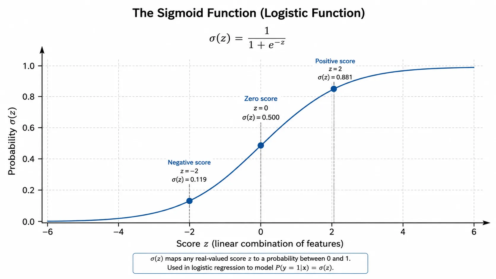
The sigmoid function converts the unrestricted linear output into a value between 0 and 1:
p = 1 / (1 + e⁻ᶻ)
The resulting curve has an S-like shape.
When the raw score is a large positive number, the predicted probability moves close to 1. When the score is strongly negative, the probability moves close to 0. When the raw score is exactly 0, the predicted probability becomes 0.5.
For example:
A raw score of 3 may produce a probability close to 0.95.
A raw score of 0 produces a probability of 0.50.
A raw score of −3 may produce a probability close to 0.05.
The sigmoid function does not simply cut off values that fall outside the probability range. Instead, it smoothly compresses every possible real number into the interval between 0 and 1.
That smooth transformation is important because it allows the model to learn gradual changes in probability rather than making abrupt jumps.
The raw linear score is also connected to the log-odds of the predicted outcome. This relationship is the main reason the method is still called regression even though its final purpose is classification. ##
An Intuitive Picture
Imagine an online learning platform trying to predict whether a student will complete a course.
The platform collects features such as:
lessons completed during the first week,
average session duration,
number of practice exercises attempted,
days since the last login,
quiz performance,
and whether the student enabled reminders.
A linear combination of these features might produce a raw score of 2.4 for one learner and −1.3 for another.
These raw scores do not have a clear business meaning. After passing them through the sigmoid function, however, the first score becomes a probability of approximately 0.92, while the second becomes approximately 0.21.
The model’s output can now be interpreted more practically:
The first learner has an estimated 92% probability of completing the course.
The second learner has an estimated 21% probability of completing it.
The learning platform can use these probabilities to design different interventions.
It might provide additional learning support to students whose completion probability falls below 40%. Students between 40% and 70% might receive reminders or motivational messages. Highly engaged students might not need any intervention.
This example reveals an important principle:
The model’s prediction and the business decision are not the same thing.
Logistic regression estimates a probability. A person, product team, medical professional, fraud analyst, or downstream software system decides what action should be taken based on that probability.
The Classification Threshold Is Not Always 0.5
One of my earliest mistakes was assuming that 0.5 was a universal classification rule.
It is not.
A threshold of 0.5 is convenient and commonly used, but it is only a default starting point. The right threshold depends on the problem and, more importantly, on the consequences of making the wrong prediction.
Consider a fraud detection system.
Missing a fraudulent payment may cost the company far more than temporarily reviewing a legitimate transaction. In this situation, the company might lower the threshold from 0.5 to 0.3.
A transaction with a fraud probability of 0.36 would then be flagged for review.
Lowering the threshold may help detect more fraudulent payments, but it will probably create more false alarms as well. Some legitimate transactions will be sent for review even though they are not fraudulent.
Now consider a system that recommends an expensive or invasive medical procedure.
A medical team might require stronger evidence before triggering that recommendation. The classification threshold could therefore be raised from 0.5 to 0.8.
This change may reduce false positive recommendations, but it can also cause the system to miss some genuine cases.
There is no threshold that automatically works best for every situation.
The correct choice depends on questions such as:
What is the cost of a false positive?
What is the cost of a false negative?
Is missing a positive case more dangerous than creating a false alarm?
How many predictions can a human team manually review?
Does the model’s predicted probability accurately reflect real-world probability?
This is why accuracy alone is rarely enough to evaluate logistic regression.
Metrics such as precision, recall, F1 score, ROC-AUC, PR-AUC, calibration, and the confusion matrix help us understand different parts of the model’s behaviour.
We will examine these metrics in detail later in the article.
Logistic Regression Is Simple, Not Weak
Because logistic regression is often taught before decision trees, random forests, gradient boosting, and neural networks, beginners sometimes assume that it is merely a classroom algorithm.
That assumption is a mistake.
Its simplicity is one of its greatest strengths.
Logistic regression is generally fast to train, easy to test, capable of producing probability estimates, and more interpretable than many complicated machine learning models. Its coefficients can help us understand how changes in individual features affect the predicted log-odds of an outcome.
Modern implementations can also support:
binary classification,
multiclass classification,
dense and sparse datasets,
L1 regularization,
L2 regularization,
Elastic-Net regularization,
and different optimization solvers.
The exact options depend on the implementation and solver being used. Scikit-learn, for example, applies regularization by default and supports several configurations for binary and multiclass logistic regression. Logistic regression is also one of the most useful baseline models.
Before building a complicated neural network or boosting pipeline, it is often worth training a properly prepared logistic regression model. It can quickly reveal whether the available features contain a useful linear signal.
Suppose a highly complex model improves validation performance by only a tiny amount but becomes slower, more expensive, and much harder to explain. In that case, logistic regression may still be the better production choice.
A strong machine learning solution is not always the model with the greatest complexity.
Sometimes, it is the simplest model that performs reliably, can be monitored easily, and allows the people using it to understand why a prediction was made.
Understanding Odds and Log-Odds
To understand logistic regression properly, we need to move beyond probability for a moment and look at odds.
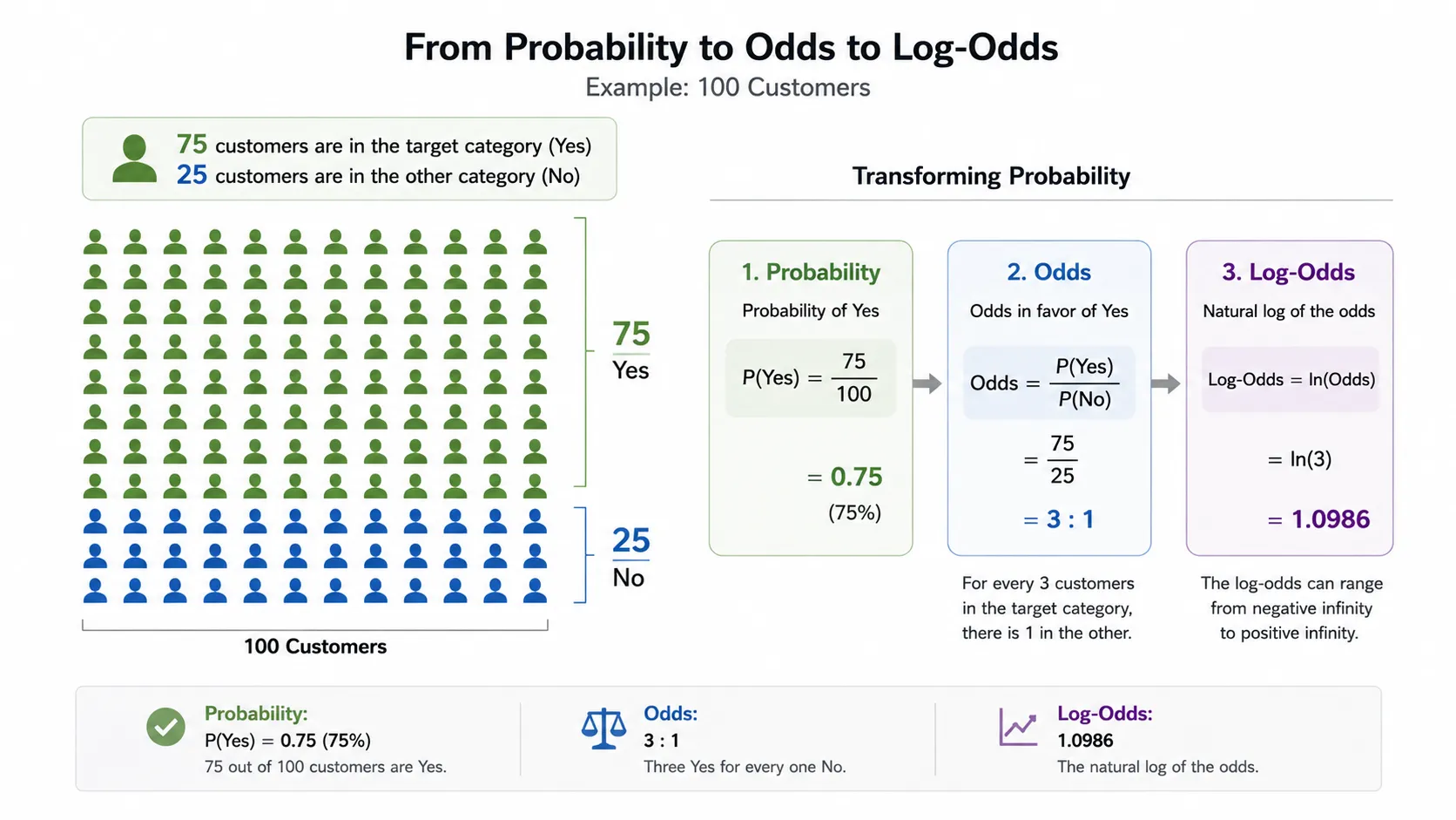
Probability tells us how likely an event is to happen. Odds compare the probability of an event happening with the probability of it not happening.
The relationship can be written as:
Odds = p / (1 − p)
Suppose a customer has a 75% probability of cancelling a subscription.
The probability of cancellation is 0.75, while the probability of not cancelling is 0.25.
The odds are:
0.75 / 0.25 = 3
This means the odds of cancellation are three to one.
Now suppose the probability of cancellation is 0.20.
The odds become:
0.20 / 0.80 = 0.25
In this case, cancellation is less likely than retention.
Odds can range from zero to positive infinity, but they are still not suitable for a linear model. A linear equation can produce negative values, while odds can never be negative.
Logistic regression solves this problem by taking the natural logarithm of the odds.
This produces the log-odds, also known as the logit:
log(p / (1 − p))
The log-odds can take any value from negative infinity to positive infinity. That makes them compatible with the unrestricted output of a linear equation.
The core logistic regression equation can therefore be written as:
log(p / (1 − p)) = b₀ + b₁x₁ + b₂x₂ + … + bₙxₙ
This equation is the mathematical heart of logistic regression.
The model assumes that the input features have a linear relationship with the log-odds of the outcome, not necessarily with the probability itself.
That difference is easy to miss, but it explains why the probability curve is not a straight line.
How Logistic Regression Coefficients Work
Each feature in logistic regression receives a coefficient.
A positive coefficient increases the log-odds of the positive outcome, while a negative coefficient decreases them.
Imagine we are building a model to predict whether a customer will cancel a software subscription.
The model uses the following features:
number of support complaints,
days since the last login,
monthly subscription price,
account age,
and number of features used regularly.
Suppose the coefficient for support complaints is positive.
This indicates that, according to the patterns in the training data, more complaints are associated with a higher probability of cancellation.
Now suppose the coefficient for account age is negative.
This may suggest that long-term customers are less likely to leave than recently acquired customers, assuming the other variables remain constant.
The phrase “assuming the other variables remain constant” is important.
A logistic regression coefficient represents the relationship between one feature and the target while holding the remaining included features fixed.
This does not automatically prove that the feature causes the outcome.
For example, a high number of support complaints may be associated with customer churn, but the complaints may not be the original cause. Poor product performance, billing errors, service outages, or unmet expectations may be creating both the complaints and the cancellation.
Logistic regression can reveal useful statistical relationships, but human reasoning is still required before turning those relationships into causal conclusions.
Interpreting Coefficients Using Odds Ratios
Raw coefficients are expressed in log-odds, which are not always intuitive.
To make them easier to interpret, we can exponentiate a coefficient:
Odds Ratio = eᵇ
Suppose the coefficient for support complaints is 0.7.
The odds ratio is approximately:
e⁰·⁷ ≈ 2.01
This suggests that a one-unit increase in the number of complaints is associated with approximately twice the odds of cancellation, assuming the other model features remain unchanged.
Now suppose another feature has a coefficient of −0.4.
Its odds ratio is approximately:
e⁻⁰·⁴ ≈ 0.67
This means a one-unit increase in that feature multiplies the odds by approximately 0.67, which represents a reduction in the odds.
However, coefficient interpretation depends heavily on the unit of measurement.
A one-unit increase in annual income is very different if income is measured in dollars, thousands of dollars, or lakhs. Similarly, a one-unit increase in account age may represent one day, one month, or one year.
Before comparing coefficients or presenting them to stakeholders, it is essential to understand how every feature has been encoded and scaled.
How Does Logistic Regression Learn?
Logistic regression learns by finding the coefficient values that make the observed training outcomes most probable.
This process is commonly explained using maximum likelihood estimation.
Suppose a training dataset contains 1,000 customers. For each customer, we know whether they actually cancelled their subscription.
The model predicts a probability for every customer.
For a customer who actually cancelled, a good model should assign a probability close to 1.
For a customer who stayed, a good model should assign a probability close to 0.
The training process adjusts the coefficients so that the probabilities assigned to the observed outcomes become as likely as possible across the complete dataset.
If a customer cancelled and the model predicted a cancellation probability of 0.95, the prediction contributes positively to the model’s likelihood.
If the customer cancelled but the model predicted a probability of 0.02, the prediction contributes very poorly.
Rather than directly maximizing likelihood in its original multiplied form, implementations normally work with logarithms. This is computationally more stable and transforms multiplication into addition.
The negative version of this objective leads us to the loss function commonly called log loss or binary cross-entropy.
Understanding Log Loss
Log loss measures how closely the predicted probabilities match the actual outcomes.
For a single observation, the binary log loss equation is:
Loss = −[y log(p) + (1 − y) log(1 − p)]
Here:
y is the actual class, either 0 or 1.
p is the predicted probability of class 1.
The equation may initially look complicated, but its behaviour is straightforward.
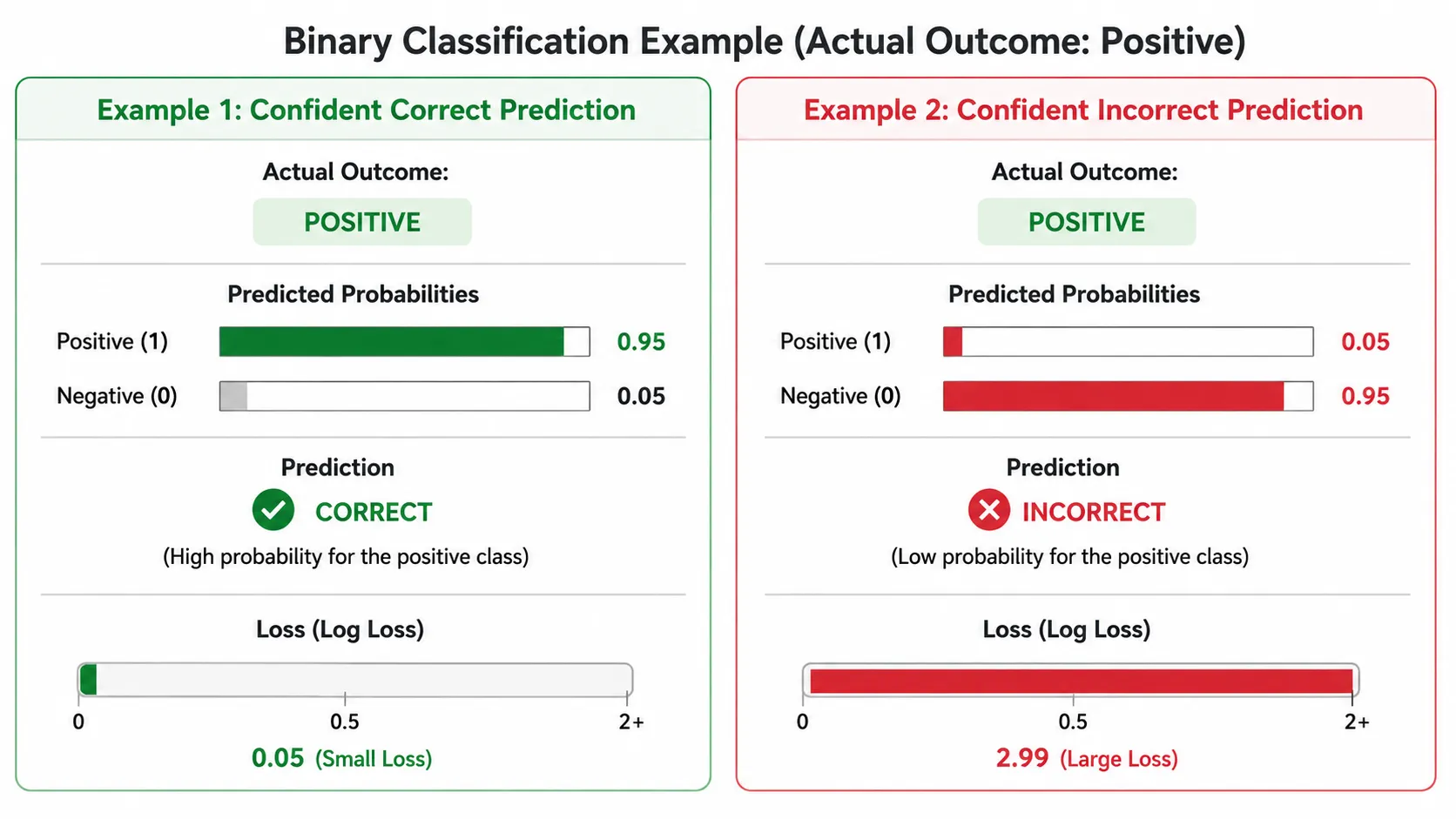
Suppose the actual result is 1.
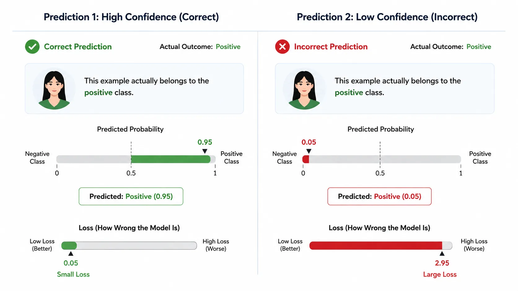
If the model predicts 0.90, the loss is small because the model assigned a high probability to the correct outcome.
If the model predicts 0.55, the loss is higher because the prediction is uncertain.
If the model predicts 0.01, the loss becomes extremely large because the model was confidently wrong.
This is one of the most valuable properties of log loss.
It does not only check whether the final class was correct. It also evaluates the quality of the probability behind the decision.
Consider two models evaluating the same positive example.
The first model predicts a probability of 0.51.
The second model predicts a probability of 0.99.
With a threshold of 0.5, both models produce the correct class. Accuracy treats them as equally correct.
Log loss does not.
The second prediction receives a lower loss because it placed much more probability on the true outcome.
Now imagine both models are wrong.
The first predicts 0.49 for a positive example, while the second predicts 0.01.
Again, accuracy treats both predictions as incorrect.
Log loss penalizes the second model much more heavily because it was not merely wrong; it was extremely confident in the wrong answer.
Why Mean Squared Error Is Usually Not Used
A natural question is why logistic regression does not simply use mean squared error, especially since it is commonly used in linear regression.
Mean squared error compares the actual value with the prediction and squares the difference.
Although it can technically be applied in some classification settings, it is not the natural objective for standard logistic regression.
The combination of the sigmoid function and log loss produces an optimization problem with useful mathematical properties. It is aligned with maximum likelihood estimation for a Bernoulli-distributed binary target and gives strong penalties to confident incorrect predictions.
Log loss also provides more informative probability learning than a metric that focuses only on the numerical distance between the label and prediction.
This is why logistic regression training usually minimizes log loss rather than the squared error used in ordinary linear regression.
Gradient Descent and Optimization
Once we define a loss function, the model needs a way to reduce it.
The training algorithm begins with initial coefficient values. It calculates predictions, measures the loss, and determines how each coefficient contributed to that loss.
The gradient tells the optimizer the direction in which the coefficients should move to reduce the error.
The coefficients are then updated repeatedly.
The process looks like this:
Initialize coefficients → Calculate probabilities → Measure loss → Calculate gradients → Update coefficients → Repeat
The learning rate controls how large each update should be.
If the learning rate is too small, training may progress very slowly.
If it is too large, the optimizer may overshoot useful coefficient values and fail to converge properly.
In practical machine learning libraries, we do not always use basic gradient descent directly. Different solvers may use methods such as limited-memory BFGS, Newton-based optimization, coordinate descent, or variance-reduced gradient techniques.
The solver choice can affect training speed, memory usage, multiclass support, and compatibility with different regularization methods.
For beginners, the default solver often works well. However, for large datasets, sparse features, multiclass problems, or specific regularization requirements, solver selection becomes important.
Why Feature Scaling Can Matter
Logistic regression does not always require feature scaling in the same way that distance-based algorithms do, but scaling can still make a major difference during optimization.
Imagine a model with two features:
annual income ranging from 200,000 to 5,000,000,
and number of support complaints ranging from 0 to 10.
The income feature operates on a much larger numerical scale.
Without scaling, the optimizer may take uneven steps across different coefficient directions, making convergence slower or less stable.
Standardization transforms a feature so that it has a mean close to zero and a standard deviation close to one.
This does not necessarily improve the underlying information in the feature, but it can help the optimization process and make regularization behave more consistently across variables.
Scaling is especially important when:
features have very different numerical ranges,
regularization is being used,
gradient-based solvers converge slowly,
or coefficients need to be compared more meaningfully.
The scaler must be fitted only on the training data.
Fitting a scaler on the complete dataset before creating the train-test split leaks information from the test data into the training process. This can make evaluation results look better than they truly are.
The safest approach is to place preprocessing and logistic regression inside a machine learning pipeline.
The Overfitting Problem
A logistic regression model can overfit when it learns patterns that work extremely well on the training data but fail to generalize to unseen examples.
This can happen when the dataset has too many features, too little training data, highly correlated inputs, noisy variables, or rare categories that appear only a few times.
Suppose a customer churn dataset contains 500 customers but 2,000 engineered features.
A model may find combinations that perfectly separate the training examples. However, many of those patterns may be accidental rather than repeatable.
The model can become overly sensitive to small changes in the input data.
Regularization helps control this behaviour by adding a penalty for excessively large coefficients.
Instead of minimizing only prediction loss, the model minimizes:
Prediction Loss + Regularization Penalty
This encourages the model to find a balance between fitting the training data and keeping the coefficients under control.
L1 and L2 Regularization
L2 regularization penalizes the squared magnitude of the coefficients.
It usually shrinks coefficients toward zero but does not force most of them to become exactly zero.
L2 is often a strong default when many features contribute small amounts of useful information.
L1 regularization penalizes the absolute magnitude of the coefficients.
It can force some coefficients to become exactly zero, effectively removing certain features from the model.
This makes L1 useful when the dataset contains many irrelevant or redundant variables.
Elastic-Net combines both L1 and L2 penalties.
It can provide feature selection through L1 while maintaining some of the stability offered by L2.
The strength of regularization is controlled through a hyperparameter. In many implementations, this parameter is represented using C, which is the inverse of regularization strength.
A smaller value of C means stronger regularization.
A larger value of C means weaker regularization.
This inverse relationship often causes confusion.
When C is extremely large, the model receives very little regularization and may fit the training data more aggressively.
When C is very small, coefficients are pushed more strongly toward zero, which may reduce overfitting but can also lead to underfitting.
The best value should be selected using validation data or cross-validation rather than guessed from the training accuracy.
Regularization Does Not Replace Good Feature Design
Regularization is useful, but it cannot repair every data problem.
If an important relationship is missing from the features, regularization cannot create it.
If the labels are incorrect, the model will still learn from incorrect information.
If the training data does not represent the real production population, the model may fail after deployment.
If a feature directly leaks information about the target, regularization does not make the evaluation trustworthy.
A reliable logistic regression model still depends on:
meaningful features,
clean labels,
representative data,
correct train-validation-test separation,
suitable evaluation metrics,
and careful monitoring after deployment.
Building a Logistic Regression Model in Python
Understanding the mathematics behind logistic regression is valuable, but the model becomes much clearer when we build one ourselves.
For this example, imagine that we are working with a subscription-based company. The company wants to predict whether a customer is likely to cancel their subscription.
Our dataset contains information such as:
monthly spending,
number of support complaints,
account age,
login frequency,
days since the last login,
and whether the customer eventually cancelled.
The target column contains two values:
0 means the customer stayed.
1 means the customer cancelled.
Before training the model, we divide the data into features and the target.
import pandas as pd
data = pd.read_csv("customer_churn.csv")
X = data.drop("cancelled", axis=1)
y = data["cancelled"]
Here, X contains the information the model will use to make predictions, while y contains the actual outcomes.
However, we should not train and evaluate the model on the same data.
A model can memorize patterns in its training dataset and still perform poorly when it receives new customer records. To estimate how well it may generalize, we divide the dataset into training and testing portions.
from sklearn.model_selection import train_test_split
X_train, X_test, y_train, y_test = train_test_split(
X,
y,
test_size=0.20,
random_state=42,
stratify=y
)
The training data is used to learn the coefficients. The test data remains unseen until evaluation.
The stratify argument helps preserve approximately the same class distribution in both datasets. This is particularly useful when one class appears much less frequently than the other.
Creating a Preprocessing and Training Pipeline
Feature scaling can improve optimization and help regularization treat numerical variables more consistently.
Instead of scaling the complete dataset before splitting it, we can place preprocessing and logistic regression inside a pipeline.
from sklearn.pipeline import Pipeline
from sklearn.preprocessing import StandardScaler
from sklearn.linear_model import LogisticRegression
model = Pipeline([
("scaler", StandardScaler()),
("classifier", LogisticRegression(
max_iter=1000,
random_state=42
))
])
model.fit(X_train, y_train)
The pipeline ensures that the scaler learns its mean and standard deviation only from the training data.
When test records are evaluated, the same transformation learned from the training set is applied to them. This prevents test data from influencing the training process.
After fitting the model, we can generate class predictions:
y_pred = model.predict(X_test)
We can also retrieve predicted probabilities:
y_probability = model.predict_proba(X_test)[:, 1]
The first output gives final classes such as 0 and 1.
The second output gives the predicted probability of the positive class. These probabilities are often more useful because they allow us to change the classification threshold according to the business problem.

Why Accuracy Can Be Misleading
Suppose our test dataset contains 1,000 customers.
Only 50 customers cancel their subscriptions, while the remaining 950 stay.
A model that predicts “will stay” for every customer achieves 95% accuracy.
At first glance, 95% appears excellent.
In reality, the model failed to identify every customer who cancelled.
This is the class imbalance problem.
When one class is much more common than the other, accuracy can hide serious weaknesses. We need evaluation metrics that examine the model from different angles.
Understanding the Confusion Matrix
The confusion matrix divides predictions into four groups:
True Positive: The model predicted cancellation, and the customer actually cancelled.
True Negative: The model predicted retention, and the customer stayed.
False Positive: The model predicted cancellation, but the customer stayed.
False Negative: The model predicted retention, but the customer cancelled.
We can calculate the confusion matrix using:
from sklearn.metrics import confusion_matrix
matrix = confusion_matrix(y_test, y_pred)
print(matrix)
The importance of each error depends on the application.
In customer churn prediction, a false positive may cause the company to send an unnecessary retention offer.
A false negative may be more expensive because the company fails to intervene before a valuable customer leaves.
In another problem, the cost relationship may be completely different.
For example, in spam detection, a false positive may send an important email to the spam folder. That mistake could be more damaging than allowing one promotional message into the inbox.
Evaluation should therefore begin with the real-world consequences of incorrect predictions, not with whichever metric produces the highest number.
Precision and Recall
Precision answers the question:
Of all the examples predicted as positive, how many were actually positive?
from sklearn.metrics import precision_score
precision = precision_score(y_test, y_pred)
High precision means the model produces relatively few false positives.
Precision becomes important when acting on a positive prediction is costly, risky, or time-consuming.
For instance, suppose a fraud investigation team can manually review only a limited number of transactions. The team may prefer a high-precision model so that most flagged payments are genuinely suspicious.
Recall answers a different question:
Of all the actual positive examples, how many did the model successfully identify?
from sklearn.metrics import recall_score
recall = recall_score(y_test, y_pred)
High recall means the model produces relatively few false negatives.
Recall becomes important when missing a positive case is especially dangerous or expensive.
A disease-screening system may prioritize recall because failing to identify a potentially affected patient could have serious consequences.
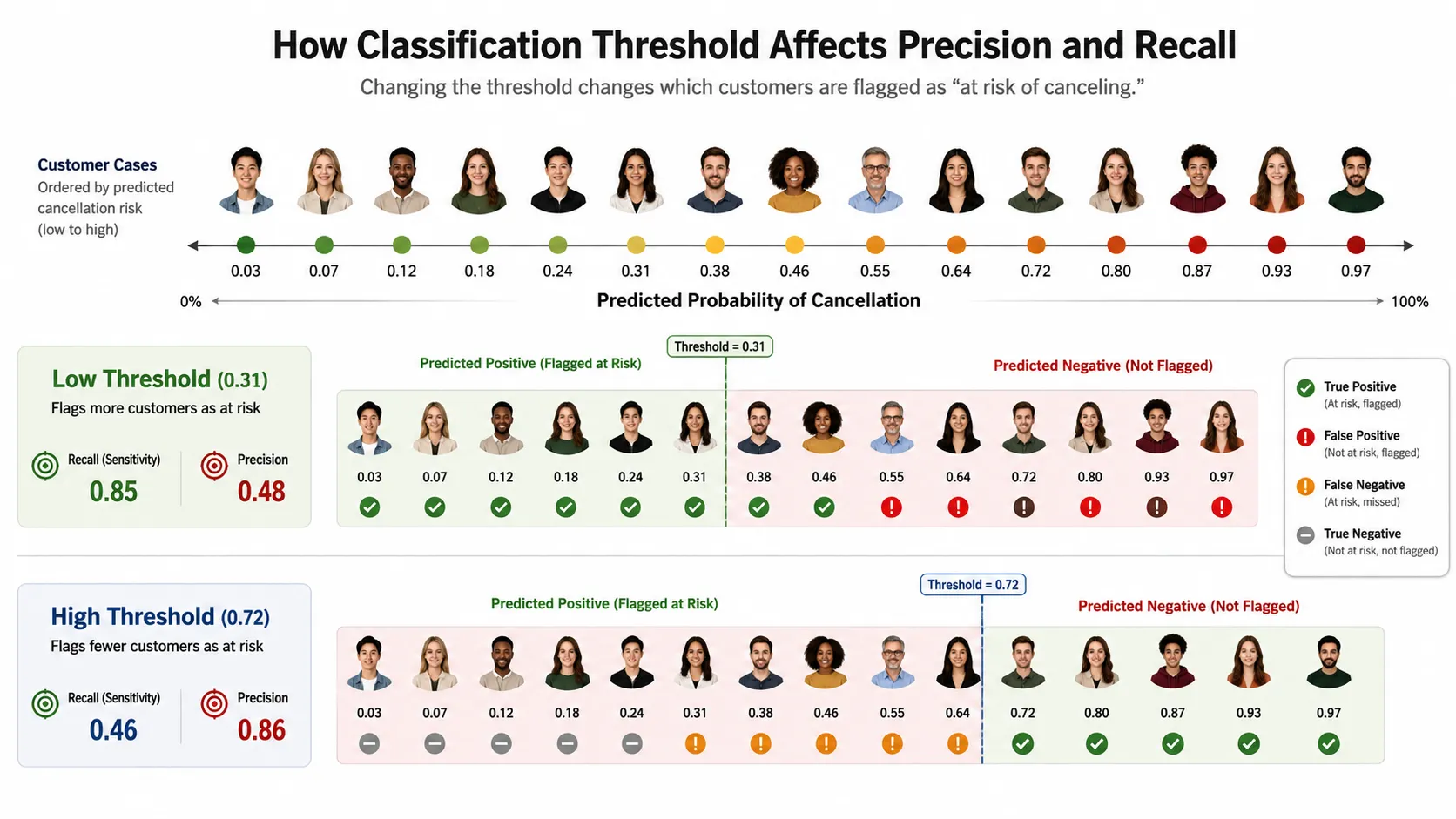
Precision and recall frequently move in opposite directions.
Lowering the classification threshold usually identifies more positive examples and increases recall. However, it may also create more false positives and reduce precision.
Raising the threshold often improves precision but may cause the model to miss more positive cases.
This is not a defect in logistic regression. It is a decision trade-off that must be aligned with the purpose of the model.
The F1 Score
The F1 score combines precision and recall using their harmonic mean.
from sklearn.metrics import f1_score
f1 = f1_score(y_test, y_pred)
The F1 score is useful when both false positives and false negatives matter and we want a single metric that balances precision and recall.
However, the F1 score should not automatically become the main evaluation metric.
It does not consider true negatives directly, and it treats precision and recall as equally important.
In real projects, the business may care far more about one type of error than the other.
For example, a customer support team may tolerate several unnecessary alerts if doing so helps identify nearly every urgent complaint. In that case, recall may be more important than a balanced F1 score.
ROC-AUC
The Receiver Operating Characteristic curve evaluates the relationship between the true positive rate and false positive rate across different classification thresholds.
ROC-AUC summarizes the curve into a single value.
from sklearn.metrics import roc_auc_score
roc_auc = roc_auc_score(y_test, y_probability)
An ROC-AUC score close to 1 indicates that the model generally ranks positive examples above negative ones.
A score close to 0.5 suggests performance similar to random ranking.
One advantage of ROC-AUC is that it evaluates model discrimination across many thresholds instead of relying only on the default threshold of 0.5.
However, ROC-AUC can sometimes appear optimistic when the positive class is extremely rare. In heavily imbalanced problems, the Precision-Recall curve may provide a more informative view.
Precision-Recall AUC
The Precision-Recall curve shows the relationship between precision and recall across thresholds.
Average Precision is commonly used to summarize performance across this curve.
from sklearn.metrics import average_precision_score
pr_auc = average_precision_score(y_test, y_probability)
PR-AUC is particularly useful when the positive class is rare and detecting it is the main objective.
Fraud detection, equipment failure prediction, security incident detection, and rare disease screening are examples where PR-AUC may reveal model quality more clearly than accuracy.
Still, no evaluation metric should be interpreted without context.
A PR-AUC value that is useful in one dataset may be inadequate in another because the class distribution, prediction difficulty, and operational costs are different.
Choosing a Better Classification Threshold
The default threshold used by many implementations is 0.5, but we can replace it.
Suppose the business wants to identify more customers who are likely to cancel. We may lower the threshold to 0.35.
custom_threshold = 0.35
custom_predictions = (
y_probability >= custom_threshold
).astype(int)
We should then recalculate precision, recall, the confusion matrix, and any business-specific cost metric using these new predictions.
custom_precision = precision_score(
y_test,
custom_predictions
)
custom_recall = recall_score(
y_test,
custom_predictions
)
custom_matrix = confusion_matrix(
y_test,
custom_predictions
)
The threshold should be selected using validation data rather than the final test set.
Repeatedly choosing a threshold based on test performance turns the test set into part of the model-development process. The final result may then look better than it will perform on genuinely unseen data.
A safer workflow is:
Training data → Learn model parameters
Validation data → Select hyperparameters and threshold
Test data → Perform final unbiased evaluation
For smaller datasets, cross-validation can provide a more reliable estimate than a single validation split.
Evaluating Probability Calibration
A classification model can rank examples correctly while still producing misleading probabilities.
Suppose a model assigns probabilities close to 0.80 to 100 customers.
If the model is well calibrated, approximately 80 of those customers should experience the predicted event.
If only 45 customers experience it, the model is overconfident.
Calibration matters whenever predicted probabilities are used for decision-making, pricing, risk estimation, resource allocation, or expected-value calculations.
A business may take different actions at probabilities of 0.20, 0.50, and 0.90. Those actions are only sensible when the probabilities have a meaningful connection to real-world event frequency.
Calibration can be examined using calibration curves and metrics such as the Brier score.
from sklearn.metrics import brier_score_loss
brier_score = brier_score_loss(
y_test,
y_probability
)
A lower Brier score generally indicates that predicted probabilities are closer to actual binary outcomes.
However, calibration should be evaluated on unseen data and monitored after deployment because real-world behaviour can change over time.
Common Logistic Regression Mistakes
One of the most common mistakes is evaluating the model on the same data used for training.
Another is preprocessing the complete dataset before creating the train-test split. This introduces data leakage.
A third mistake is treating accuracy as proof that the model is useful.
Other practical problems include:
ignoring class imbalance,
using the default threshold without analysing its consequences,
including target leakage features,
failing to handle missing values,
interpreting correlation as causation,
comparing coefficients with different measurement scales,
ignoring interactions between variables,
and assuming predicted probabilities are automatically calibrated.
Data leakage can be particularly difficult to notice.
Suppose we are predicting customer cancellation and include a feature called account_closed_date. That feature may make the model appear highly accurate because it directly reveals information that becomes available only after cancellation.
The model is not predicting the future. It is reading evidence from the future.
A reliable feature should be available at the exact moment the prediction will be made in production.
When Logistic Regression Works Well
Logistic regression is a strong choice when the relationship between the features and the log-odds is reasonably linear.
It performs particularly well when:
the dataset is not excessively noisy,
features have meaningful predictive signals,
interpretability is important,
training speed matters,
probability estimates are required,
or a strong baseline model is needed.
It can also work effectively with high-dimensional sparse data, such as text features created using bag-of-words or TF-IDF representations.
However, logistic regression may struggle when the true decision boundary is highly nonlinear.
Suppose loan risk depends on a complicated interaction between income, age, employment type, debt ratio, location, and economic conditions. A basic logistic regression model may not capture that structure unless the relevant transformations and interaction features are added.
Decision trees, gradient-boosting models, kernel methods, or neural networks may perform better in such cases.
Even then, logistic regression remains valuable as a baseline. If a complicated model cannot meaningfully outperform it on properly validated data, the added complexity may not be justified.
From Notebook Accuracy to Production Reality
A model that performs well in a notebook is not automatically ready for production.
The data entering the live system must be processed in exactly the same way as the training data.
Feature definitions must remain consistent.
Missing values and unexpected categories must be handled safely.
Prediction latency should meet the application’s requirements.
The classification threshold must reflect operational capacity.
Most importantly, the model must be monitored after deployment.
Customer behaviour can change. Fraud patterns can evolve. Marketing campaigns may alter purchasing habits. A new product feature may change the meaning of existing variables.
This change is often called data drift or concept drift.
A production monitoring system should track:
feature distributions,
prediction distributions,
missing-value rates,
class balance,
model discrimination,
probability calibration,
business outcomes,
and threshold-based alert volume.
Logistic regression is mathematically elegant, but its real value depends on everything around it: data quality, validation design, threshold selection, monitoring, and the decisions made from its predictions.
The model does not understand customers, diseases, fraud, or risk in the way a human expert does.
It identifies statistical patterns in historical data.
Our responsibility is to verify whether those patterns are reliable, relevant, fair, and useful before allowing them to influence real decisions.


