


Imagine that one of your friends asks you whether they should carry an umbrella today.
You probably would not answer immediately. You might first check whether the sky is cloudy. Then you may look at the weather forecast. You may also consider the season, the chance of rain, and how long your friend will stay outside.
Without realizing it, you have followed a series of simple questions before reaching a decision.
A decision tree works in a very similar way.
It takes a large problem, divides it into smaller questions, and follows the answers until it reaches a final prediction. A random forest takes this idea one step further. Instead of depending on one decision tree, it creates many trees and combines their answers.
That is the basic idea behind two of the most useful machine learning algorithms.
In this guide, we will understand decision trees and random forests through everyday situations, simple language, and practical examples. You do not need advanced mathematics or programming experience. You only need to understand how one question can lead to another.
What Is a Decision Tree in Machine Learning?
A decision tree is a supervised machine learning algorithm that makes predictions by dividing data into smaller groups.
It can be used for both classification and regression problems. Classification means predicting a category, while regression means predicting a numerical value. a decision tree may be used to predict:
Whether an email is spam or not
Whether a customer will buy a product
Whether a loan applicant is high-risk or low-risk
What the expected price of a house could be
How much a customer may spend next month
The algorithm does not study all the information at once. It starts with one question and gradually moves toward the answer.
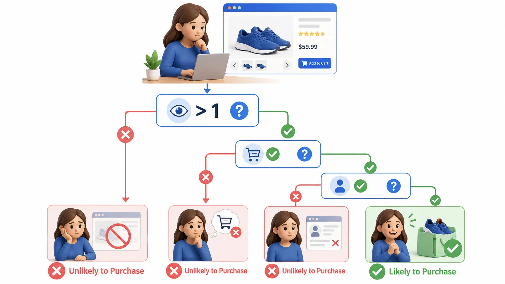
Think about an online shopping website trying to predict whether a visitor will purchase a pair of shoes.
The tree may begin with this question:
Has the visitor viewed the product more than once?
If the answer is no, the visitor may be less likely to buy.
If the answer is yes, the tree may ask another question:
Has the visitor added the shoes to the cart?
If the answer is yes, it may then check whether the visitor has previously purchased something from the website.
Each answer moves the visitor through a different path. At the end of that path, the model produces a prediction such as:
Likely to purchase or unlikely to purchase.
Why Is It Called a Decision Tree?
The structure of this algorithm looks similar to an upside-down tree.
It begins with one main question at the top. That question creates different paths or branches. Each branch can lead to another question, and the process continues until the model reaches a final answer.
A decision tree has three main parts.
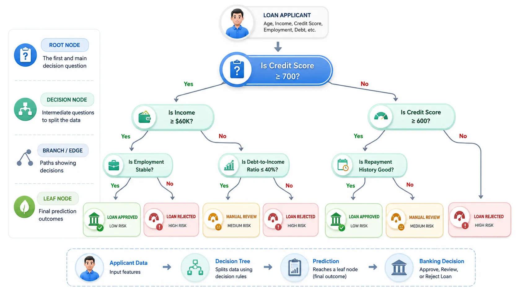
Root Node
The root node is the first question asked by the model.
It is placed at the top of the tree and usually represents the feature that can divide the data most effectively.
In a loan approval example, the first question might be:
Is the applicant’s monthly income above a certain amount?
This question creates the first major division in the data.
Decision Nodes
Decision nodes are the questions that appear after the root node.
Suppose the applicant’s income is above the required amount. The next question may be:
Does the applicant have a good credit history?
Another question could be:
Is the existing debt within an acceptable limit?
Every decision node helps the model understand the case more clearly.
Leaf Nodes
A leaf node is the final result of a path.
Once the model reaches a leaf node, it stops asking questions and produces its prediction.
In the loan example, the final result could be:
Approve the loan
or:
Reject the loan
A leaf node can also contain a numerical prediction. For example, in a house-price prediction model, the final leaf may show an estimated price of ₹65 lakh.
A Real-Life Decision Tree Example
Let us understand the complete process through a familiar situation.
Suppose you are deciding whether to order food from a restaurant.
Your first question may be:
Are you hungry?
If the answer is no, you do not order food.
If the answer is yes, you ask:
Is food already available at home?
If food is available, you may eat at home. If it is not available, you move to the next question:
Is the delivery time less than 30 minutes?
If the delivery is quick, you place the order. If it takes too long, you may choose another restaurant or cook something yourself.
This is exactly how a decision tree turns one large decision into several smaller decisions.
The machine learning model follows the same process, but instead of creating questions from personal experience, it learns useful questions from historical data.
For example, a food delivery company may study previous orders and use information such as:
Time of day
Customer location
Delivery fee
Restaurant rating
Previous order history
Estimated delivery time
Available discounts
The model examines these factors and learns which questions help it make better predictions.
Classification and Regression in Decision Trees
Decision trees can solve two major types of prediction problems.
Decision Tree Classification
Classification is used when the expected answer belongs to a category.
If you are new to classification models, check out our step-by-step guide on Logistic Regression to understand how linear binary classification works.
For example:
Fraud or genuine transaction
Pass or fail
Customer will leave or stay
Product will be returned or kept
Disease detected or not detected
Imagine a bank trying to identify a suspicious card transaction.
The tree may ask whether the purchase amount is unusually high. It may then check whether the transaction happened in a new location or on an unfamiliar device. Based on these answers, the transaction may be classified as normal or potentially fraudulent.
Decision Tree Regression
Regression is used when the answer is a numerical value.
Unlike Logistic Regression, which uses a straight-line formula to predict numbers, decision tree regression splits data into ranges to estimate values.
For example:
House price
Monthly sales
Delivery time
Electricity consumption
Expected customer spending
Suppose a property platform wants to estimate the price of a house. The decision tree may consider the location, area, number of rooms, property age, nearby facilities, and previous selling prices.
Different houses follow different branches of the tree. At the end, the model provides an estimated price instead of a category.
This ability to handle both categories and numbers makes decision trees useful for many practical machine learning problems.
How Does a Decision Tree Learn?
A decision tree learns by searching for questions that divide the available data into meaningful groups.
Suppose a school has data about students’ attendance, study hours, assignment scores, and final results. The model may discover that study hours create the clearest first division.
It might begin with:
Does the student study for more than two hours per day?
After creating the first split, the model studies each group separately and searches for the next useful question.
The process continues until the model reaches a stopping point or produces groups that are clear enough for prediction.
However, every possible question is not equally useful. The model needs a way to measure which split creates the cleanest and most meaningful groups. This is where ideas such as Gini impurity, entropy, and information gain become important.
These terms may sound technical, but their purpose is simple: they help the model choose the best question at each stage.
How Does a Decision Tree Choose the Best Question?
A decision tree can create many possible questions from the available data. However, asking random questions would not produce a useful model.
The tree must find the question that separates the data in the clearest possible way.
Suppose we have data from 100 customers who visited an online store. Out of these customers, 40 purchased a product and 60 left without purchasing anything.
The dataset contains information such as:
Time spent on the website
Number of product pages viewed
Whether a product was added to the cart
Whether the customer used a discount coupon
Previous purchase history
The model may try several questions:
Did the customer spend more than five minutes on the website?
Did the customer view more than three products?
Did the customer add something to the cart?
Each question divides customers into different groups. The decision tree checks which question creates groups where customers are more similar to one another.
For example, if most customers who added a product to the cart completed the purchase, this question creates a useful split. It helps separate likely buyers from visitors who are less likely to buy.
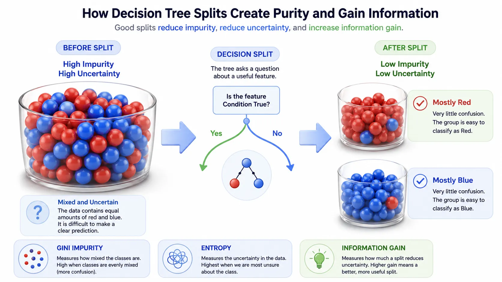
To compare these possible splits, decision tree algorithms commonly use measurements such as Gini impurity, entropy, and information gain.
What Is Gini Impurity?
Gini impurity measures how mixed a group of data is.
Imagine two boxes containing red and blue balls.
The first box contains only red balls. Because every ball belongs to the same group, the box is completely pure.
The second box contains an equal number of red and blue balls. Since both types are mixed together, the box has high impurity.
A decision tree prefers splits that create purer groups.
Let us connect this idea with a real business example.
Suppose an online learning platform wants to predict whether a student will complete a course. After checking the data, the model divides students based on whether they watched the first three lessons.
In the first group, almost every student completed the course.
In the second group, most students left the course early.
This would be considered a useful split because the two groups are fairly clear. One group mostly contains course completers, while the other mostly contains students who dropped out.
If both groups contained an almost equal mix of completers and non-completers, the split would not be very helpful.
Gini impurity allows the algorithm to measure this difference and choose a better question.
Entropy and Information Gain Explained Simply
Entropy is another way to measure how mixed or uncertain a dataset is.
When a group contains many different outcomes in almost equal numbers, uncertainty is high. When most data points belong to one category, uncertainty is low.
Consider a jar containing chocolates.
If every chocolate has the same flavour, you already know what you will get when you pick one. There is almost no uncertainty.
If the jar contains many flavours in equal amounts, you cannot easily guess which flavour you will pick. The uncertainty is much higher.
Entropy works with the same basic idea.
A decision tree tries to reduce this uncertainty after every question.
The reduction in uncertainty is called information gain.
Suppose a company wants to predict whether an employee will leave the organisation. Before creating a split, the dataset contains a mix of employees who stayed and employees who resigned.
The model asks:
Has the employee received a promotion in the last three years?
After this question, it may discover that employees who received a promotion usually stayed, while employees who did not receive one were more likely to leave.
The question has created clearer groups, so it provides useful information.
A split with higher information gain is usually preferred because it helps the model move closer to a reliable prediction.
How the Tree Grows Step by Step
Once the first question is selected, the same process is repeated for every new group.
Imagine a travel website trying to predict whether a user will book a hotel.
The first question may be:
Has the user selected travel dates?
Users who have not selected dates may be less ready to book. Users who have selected dates move to another question:
Has the user opened a hotel details page?
If the answer is yes, the tree may then check:
Has the user compared more than one room?
After that, it may ask whether the user has reached the payment page.
Every question creates a new branch. The tree continues growing until it reaches a final result, such as:
High chance of booking
or:
Low chance of booking
This step-by-step structure makes the decision tree algorithm easy to understand. Unlike some machine learning models that behave like a black box, a decision tree allows us to follow the path behind a prediction.
However, a tree should not continue growing forever.
If it creates too many branches, it can start memorising the training data instead of learning general patterns.
What Is Overfitting in a Decision Tree?
Overfitting happens when a model performs very well on the data it studied but struggles with new data.
Think about a student who memorises the exact answers from a practice paper without understanding the subject. If the real examination contains the same questions, the student may score well. But if the questions are slightly different, the student may struggle.
A deeply grown decision tree can face the same problem.
Suppose a tree is trained to predict whether people will buy a smartphone. A simple model may use useful factors such as budget, preferred brand, desired camera quality, and battery requirements.
An overfitted tree may create highly specific rules such as:
Customer is 27 years old
Visited the website at 8:17 PM
Viewed one particular phone four times
Used an Android device
Lives in one specific postal area
These details may perfectly describe a few people in the training data, but they may not help predict the behaviour of future customers.
The tree has learned noise instead of a useful pattern.
Overfitting is one of the biggest weaknesses of a single decision tree.
How Can Overfitting Be Controlled?
One way to control overfitting is to limit how much the tree can grow.
The model can be stopped based on conditions such as:
Maximum tree depth
Minimum number of records required to create a split
Minimum number of records required in a final leaf
Maximum number of leaf nodes
Another useful method is called pruning.
Pruning means removing branches that add complexity but do not improve predictions in a meaningful way.
It is similar to cutting unnecessary branches from a plant so that the plant can grow in a healthier and more controlled form.
Suppose a loan prediction tree contains a long branch based on very specific customer details. If removing that branch does not reduce the model’s performance, the branch may not be useful. Pruning removes it and makes the model simpler.
A smaller tree is usually easier to explain and may perform better on new data.
Still, even a well-controlled decision tree can change significantly when the training data changes slightly. One dataset may create one root question, while a slightly different dataset may create another.
This is where random forests become valuable.
What Is a Random Forest?
A random forest is a machine learning model made from many decision trees.
Instead of trusting one tree, it asks multiple trees to make a prediction and then combines their answers.
Imagine asking one friend whether you should buy a particular laptop. That friend may give useful advice, but their opinion could be influenced by personal preference.
Now imagine asking 100 people with different experiences. Some may focus on battery life, some on performance, some on price, and others on durability.
When their opinions are combined, the final decision is often more balanced.
A random forest follows a similar approach.
Each decision tree studies a slightly different sample of the training data. The trees may also consider different groups of features while choosing their questions.
As a result, the trees do not all make exactly the same mistakes.
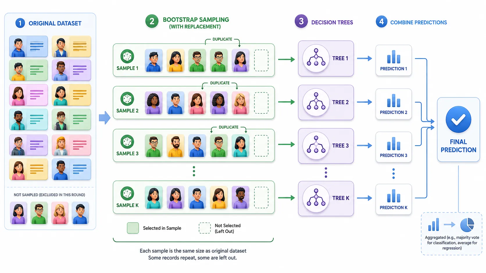
For classification, the forest usually selects the category that receives the most votes.
For regression, it usually calculates the average of the predictions produced by all trees.
A single decision tree can be simple and easy to explain, but it may be unstable or overfit the data. A random forest reduces this weakness by combining many different trees.
The next step is to understand how these trees are created, why randomness matters, and how the final prediction is calculated.
How Does a Random Forest Work?
A random forest does not simply create several identical decision trees. If every tree studied the same data and asked the same questions, they would probably make the same mistakes.
To avoid this problem, the algorithm adds randomness in two important ways.
First, every decision tree is trained on a different sample of the original dataset. Second, each tree is allowed to consider only a limited selection of features while choosing a split.
This gives every tree a slightly different view of the problem.
Suppose a bank has information about 10,000 previous loan applicants. The data includes income, age, credit score, employment type, existing loans, repayment history, and requested loan amount.
One decision tree may learn from a sample containing more salaried applicants. Another may study a sample with more self-employed applicants. A third tree may focus strongly on credit score and repayment history, while another may consider income and existing debt.
Each tree creates its own prediction.
The random forest then combines these predictions to produce a final answer.
This process makes the model more stable than a single decision tree.
Understanding Bootstrap Sampling
The method used to create different training samples is commonly known as bootstrap sampling.
Imagine a bag containing 100 numbered cards. To create one sample, you randomly pick a card, record its number, and place it back inside the bag. You then repeat the same process until you have selected 100 cards.
Because every card is returned to the bag, some cards may be selected multiple times, while others may not be selected at all.
A random forest uses a similar method with training data.
Every decision tree receives a randomly created sample. Some records may appear more than once in a tree’s training sample, while some may be left out.
This small variation helps the trees learn different patterns.
The idea of training multiple models on different samples and combining their predictions is called bagging, which stands for bootstrap aggregating.
Bagging reduces the risk that the complete model will depend too heavily on one unusual pattern in the data.
Why Are Random Features Used?
Random forest also introduces randomness while selecting features.
Suppose a dataset has ten features. A normal decision tree may examine all ten features before choosing the best split. In a random forest, each tree may be allowed to examine only a small random group of those features.
For example, one tree may compare age, income, and credit score. Another may compare employment type, repayment history, and existing debt.
This prevents one powerful feature from dominating every tree.
Consider a recruitment model where previous work experience is strongly connected with hiring decisions. If every tree always selects experience as its first question, all trees may become too similar.
By giving each tree a different group of features, the random forest encourages variety.
This variety matters because a group of different trees usually makes a more balanced decision than a group of almost identical trees.
How Is the Final Prediction Made?
The final prediction depends on whether the random forest is solving a classification or regression problem.
In random forest classification, every tree votes for a category.
Suppose 100 trees are predicting whether a customer will cancel a subscription.
Sixty-eight trees predict that the customer will stay, while thirty-two predict that the customer will leave.
The final prediction will be:
The customer is likely to stay.
In random forest regression, the model takes the average of all numerical predictions.
Imagine that several trees are estimating the price of a house. Some trees predict ₹72 lakh, some predict ₹75 lakh, and others predict ₹78 lakh.
The random forest combines these values and may produce a final estimate close to ₹75 lakh.
One tree may give an unusually high or low prediction, but its impact becomes smaller when many predictions are averaged.
Decision Tree vs Random Forest
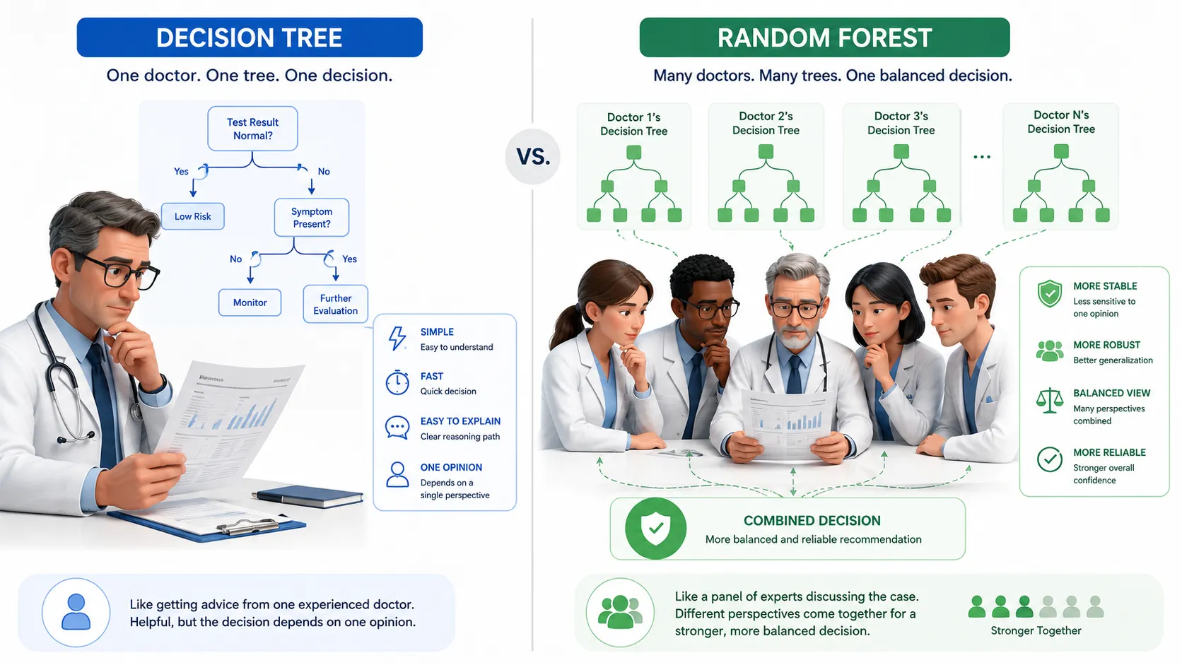
The main difference between a decision tree and a random forest is the number of trees used.
A decision tree depends on one tree. A random forest combines many decision trees.
A single decision tree is easier to understand because you can follow every question from the root node to the final leaf. This makes it useful when explanation and transparency are important.
A random forest is harder to visualise because it may contain hundreds of trees. However, it usually provides more stable and accurate predictions.
A decision tree can also overfit easily when it grows too deeply. A random forest reduces this risk by combining trees trained on different samples and feature groups.
Think of a decision tree as one experienced doctor offering an opinion. A random forest is more like a panel of doctors studying the same case from different angles and reaching a combined conclusion.
The single doctor’s reasoning may be easier to follow. The panel’s final judgement, however, may be more balanced.
Advantages of Decision Trees
Decision trees are popular because their structure is simple and visual.
They can work with both classification and regression problems. They also require less data preparation than many other machine learning algorithms.
A decision tree can capture non-linear relationships. This means it can understand patterns that do not follow a simple straight-line connection.
Its biggest advantage is interpretability.
For example, if a loan application is rejected, the tree’s path can help explain whether the decision was influenced by credit history, income, existing debt, or another factor.
However, a decision tree can become unstable. A small change in the training data may create a different tree. Deep trees may also memorise noise and perform poorly on new data.
Advantages of Random Forests
Random forests are usually more reliable than individual decision trees.
They reduce overfitting, handle large datasets, and can work with many input features. They can also estimate which features are most useful for predictions.
For example, a hotel booking company may use a random forest to predict cancellations. The model might reveal that booking time, payment type, room price, trip duration, and previous cancellation history have the strongest influence.
This information can help the company improve its policies and customer communication.
Random forests are also less affected by unusual records because their final result depends on many trees rather than one.
Their main drawback is complexity. A model containing hundreds of trees needs more computing power and is harder to explain in complete detail.
Where Are Decision Trees and Random Forests Used?
These algorithms are used in many areas of everyday life.
Banks use them for credit-risk analysis and fraud detection. Online stores use them to predict purchases and recommend products. Hospitals may use them to support disease-risk assessment. Travel platforms can use them to predict hotel cancellations, booking behaviour, or customer preferences.
They are also useful in marketing, agriculture, education, insurance, manufacturing, and cybersecurity.
A school may predict which students need extra support. A delivery company may estimate whether an order will arrive late. A farm may predict crop quality using weather, soil, and irrigation data.
The problem may change, but the basic process remains similar: study previous examples, ask useful questions, and use the learned patterns to predict future outcomes.
Which Model Should You Choose?
Choose a decision tree when the model needs to be simple, fast, and easy to explain.
It is a strong choice for learning machine learning concepts, presenting business rules, or building an initial model that acts as a clear baseline.
Choose a random forest when prediction quality and stability matter more than explaining every individual decision.
In a real project, it is often useful to test both models. Start with a decision tree, study its mistakes, and then compare its performance with a random forest.
Do not select a model only because it sounds advanced. The right choice depends on the dataset, the business problem, the need for explanation, and the cost of incorrect predictions.
Final Thoughts
Decision trees and random forests may look technical at first, but both are built around a familiar human habit: asking questions before making a decision.
A decision tree follows one organised path of questions. A random forest creates many such paths and combines their answers.
The decision tree gives simplicity and transparency. The random forest adds stability, variety, and often better prediction performance.
Once you understand roots, branches, leaf nodes, splitting, overfitting, bagging, and feature randomness, these algorithms stop feeling mysterious.
You begin to see them as structured versions of the decisions we already make every day—only faster, larger, and supported by data.


