


Imagine you run an online travel platform and want to predict whether a customer will cancel a hotel booking. You check the booking price, travel date, stay length, payment method, and customer history. A single decision tree may notice a few useful patterns, but real customer behaviour is rarely that simple.
One rule may work for weekend bookings and fail for business travellers. Another may work during holidays but become unreliable during normal weeks.
This is where gradient boosting becomes powerful.
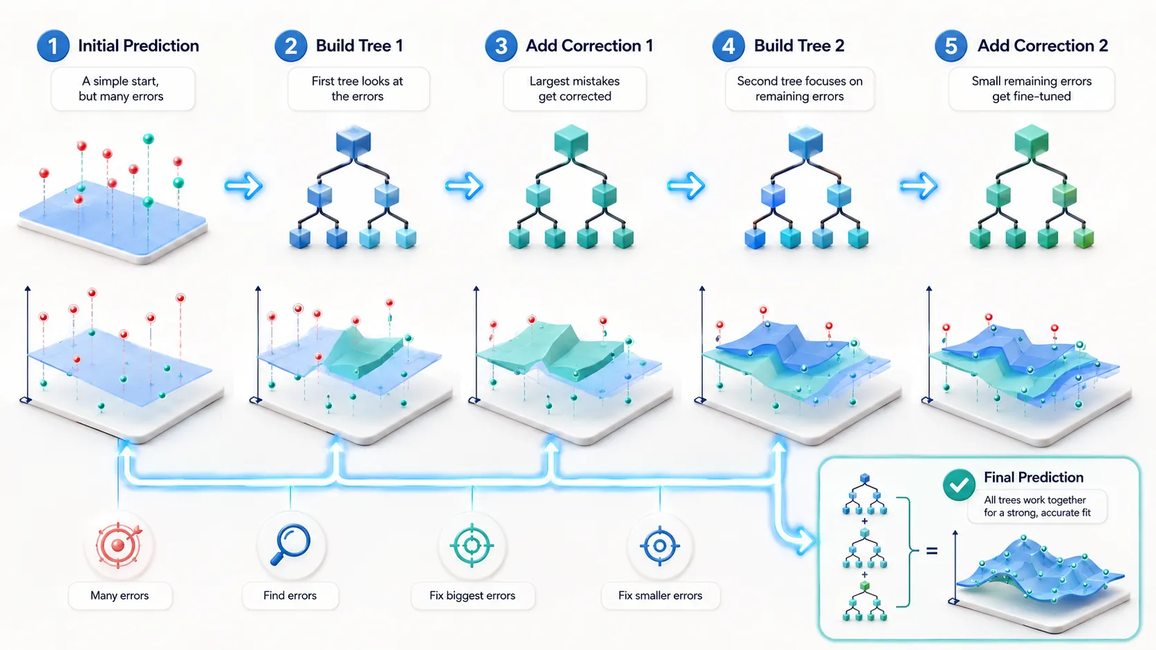
Instead of asking one large model to make a perfect prediction, gradient boosting creates a team of small decision trees. Each new tree studies the mistakes made by the trees before it and adds a correction. The final prediction is produced by combining all those small improvements.
XGBoost and LightGBM use this same core idea, but they do not build and optimize trees in exactly the same way. That difference can affect training speed, memory use, accuracy, overfitting, and the amount of tuning required.
What Is Gradient Boosting in Simple Words?
Gradient boosting is an ensemble learning method. The word “ensemble” simply means that several models work together instead of relying on only one model.
In gradient boosting, these models are usually small decision trees. They are created one after another rather than being trained independently.
The first tree makes an initial prediction. That prediction will not be perfect. The algorithm measures the errors and trains the next tree to reduce them.
A third tree then tries to fix the errors still left after the second tree. This process continues until the selected number of trees has been created or the model stops improving.
Google’s machine-learning guide describes gradient boosting as an iterative process in which each new weak model improves the current combined model. XGBoost’s official documentation explains boosted trees through the same supervised-learning idea: prediction quality improves as new trees are added while model complexity is controlled.
The word “gradient” may sound mathematical, but its basic role is simple.
It tells the model the direction in which its errors should be reduced. Think of it like a navigation signal saying:
“Your answer is too high.”
“Your answer is too low.”
“This type of example needs more attention.”
The model uses this direction to decide what the next tree should learn.
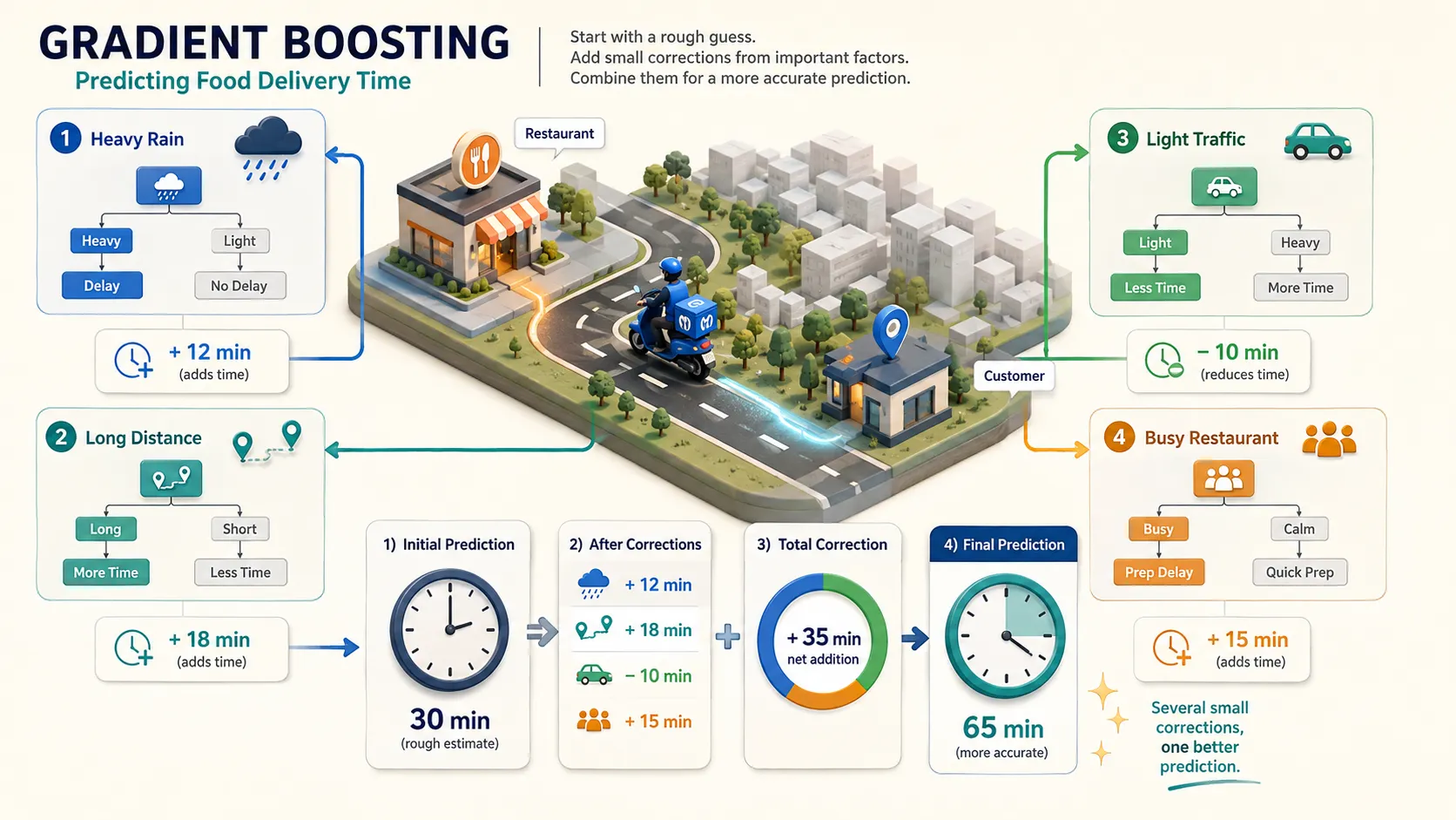
A Real-Life Example: Estimating Delivery Time
Suppose your friend asks you to predict how long a food delivery will take.
Your first answer is simple: every order will take 30 minutes.
One order actually takes 45 minutes. Your estimate was 15 minutes too low.
Another order takes only 22 minutes. Your estimate was 8 minutes too high.
These differences are the errors the model needs to learn from.
The first small decision tree may discover that orders placed during heavy rain usually take longer. It adds some extra time for rainy conditions.
The second tree may notice that restaurants located far from the customer create another delay. It adds a correction based on distance.
The third tree may learn that late-night traffic is lighter, so some orders arrive faster. It adjusts the prediction again.
Another tree may notice that a busy restaurant takes longer to prepare food, while a small nearby restaurant may complete the order quickly.
No single tree understands the complete situation.
However, rain, distance, traffic, preparation time, order size, and driver availability gradually become part of the combined prediction.
This is the basic logic of gradient boosting:
Start with a rough answer, study the mistakes, and improve that answer in small steps.
How Gradient Boosting Learns Step by Step
1. It Starts With a Basic Prediction
For a regression problem, the model may begin with an average value.
For example, if house prices in a dataset have an average value of ₹50 lakh, the first prediction for every house may be close to ₹50 lakh.
For a classification problem, the model may begin with a basic probability. At this stage, the prediction is intentionally simple.
2. It Measures the Error
The algorithm compares predicted values with actual values through something called a loss function.
A loss function is simply a scoring rule that tells the model how wrong its predictions are.
Suppose the model predicts a house price of ₹50 lakh, but the real price is ₹65 lakh. The model has made an error of ₹15 lakh.
A lower loss generally means that the predictions are closer to the expected answers.
3. It Builds a Small Tree to Correct the Error
The next decision tree focuses on the remaining mistakes.
It does not restart the entire learning process. Its job is to improve the prediction already produced by the current collection of trees.
For example, the new tree may discover that houses near a metro station are usually more expensive. It can then add a positive correction for those houses.
Another tree may learn that very old houses without renovation are generally cheaper and reduce their predicted prices.
4. It Adds a Controlled Correction
The correction produced by each new tree is usually controlled by a learning rate.
A small learning rate allows every tree to make only a limited change. This often requires more trees, but it can create a more controlled learning process.
Think of it like improving a recipe.
Instead of adding a full spoon of salt after one taste, you add a small amount, taste it again, and then make another adjustment. Smaller corrections reduce the chance of completely ruining the final result.
Google’s gradient-boosted tree guide calls this scaling approach shrinkage. It controls how strongly each new tree changes the combined model.
5. It Repeats the Process
More trees are added, and each one works on what the previous trees still failed to explain.
Training may stop after a fixed number of rounds. It may also stop when performance on validation data no longer improves.
This second method is commonly known as early stopping. It helps prevent the model from continuing to learn patterns that may only exist in the training data.
Why Not Use One Very Deep Decision Tree?
A very deep decision tree can memorize small details from the training data.
It may appear highly accurate during training but perform poorly when completely new data arrives. This problem is called overfitting.
Imagine a student who memorizes the exact answers from one practice paper but does not understand the actual subject. The student may score perfectly on the same questions but struggle when the wording changes.
A deeply overfitted decision tree can behave in a similar way.
Gradient boosting takes a different route. It combines many controlled trees, with every tree handling a smaller correction.
This does not automatically prevent overfitting. However, settings such as learning rate, tree depth, number of leaves, regularization, minimum samples, and early stopping give us different ways to control it.
This is also where XGBoost and LightGBM begin to separate.
XGBoost was designed as a scalable tree-boosting system with regularization and engineering improvements for sparse and large datasets. LightGBM uses histogram-based learning and grows trees leaf-wise, choosing the leaf that can reduce the loss the most.
LightGBM’s official documentation also warns that leaf-wise growth may overfit on smaller datasets unless tree complexity is limited carefully.
Before choosing between XGBoost and LightGBM, remember the central idea:
Both tools learn through repeated corrections.
Once this foundation is clear, understanding their differences, strengths, limitations, and ideal use cases becomes much easier.
What Is XGBoost?
XGBoost stands for Extreme Gradient Boosting. It takes the basic gradient boosting idea and adds controls that make the model more reliable on real datasets.
Think again about the food delivery example. A normal boosting model keeps adding trees to correct old mistakes. XGBoost does the same, but it also asks:
“Is this new split useful enough to justify itself?”
If the improvement is too small, the model can avoid that split. XGBoost also uses regularization, which places a penalty on unnecessary complexity. This helps reduce the risk of memorizing the training data instead of learning a useful pattern.
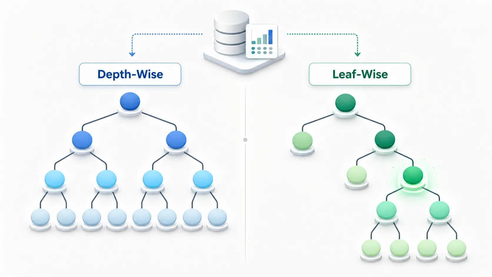
XGBoost supports different tree-building methods, including a fast histogram-based method. Its default growth policy is depth-wise, which generally expands nodes closer to the top before moving deeper. It can also use a loss-guided policy when configured for it.
This controlled style is one reason XGBoost is often a dependable starting point. It may not always train first, but it can provide stable results without aggressive tuning.
What Is LightGBM?
LightGBM stands for Light Gradient Boosting Machine. It was designed to make gradient-boosted decision trees efficient for large and high-dimensional datasets.
Its main difference appears in the way it grows a tree.
LightGBM normally uses leaf-wise growth. Instead of expanding all nodes at a similar depth, it finds the leaf where the next split can reduce the loss the most and grows that leaf first.
Imagine that a teacher has ten students but only a few minutes for revision. Instead of giving equal time to everyone, the teacher first helps the student whose mistakes can be improved the most. LightGBM follows a similar strategy.
This approach can reduce training loss quickly. However, it may create a deep branch on one side of the tree. On a small dataset, that flexibility can also make LightGBM learn noise unless settings such as num_leaves, max_depth, and min_data_in_leaf are controlled carefully.
XGBoost vs LightGBM: The Main Tree-Growth Difference
Suppose an online store wants to predict whether a customer will complete a purchase.
The data includes device type, traffic source, product price, previous orders, session time, and discount percentage.
An XGBoost model using its default depth-wise policy generally grows the tree in a more level-controlled way. After creating an important split, it continues exploring nodes closer to the current depth. The resulting tree often looks more balanced.
LightGBM asks which available leaf can create the largest improvement right now. If mobile users arriving from social media show a strong pattern, LightGBM may keep expanding that branch while leaving other branches smaller.
Neither method is automatically better.
XGBoost’s default approach can feel more controlled when the dataset is not very large. LightGBM’s leaf-wise method can learn difficult patterns quickly with enough data. But that same flexibility means tree complexity needs close attention.
Which One Is Faster?
LightGBM is often chosen when training speed and memory efficiency matter. It converts continuous values into discrete bins and builds histograms from those bins. Working with a limited number of bins reduces the calculations needed while searching for useful splits.
Its original design also introduced Gradient-based One-Side Sampling and Exclusive Feature Bundling.
GOSS gives more attention to examples with larger gradients because they carry more information about the model’s current errors.
EFB combines features that rarely have non-zero values at the same time, reducing the number of features that must be processed.
XGBoost also provides a fast histogram tree method, so the speed difference is not a permanent rule. Dataset size, number of columns, sparsity, hardware, parameter settings, and library version can all affect the result.
The more accurate conclusion is this:
LightGBM is often a strong speed-first choice for large tabular datasets, while XGBoost can be competitive and may provide a more controlled starting experience.
How Do They Handle Categorical Features?
Categorical features contain labels rather than continuous measurements. Examples include:
City
Hotel type
Payment method
Device category
Airline
Membership level
LightGBM can work with categorical features directly when they are identified correctly. It searches for useful category groupings instead of requiring every category to become a separate one-hot encoded column. This helps when a feature contains many categories.
Modern XGBoost versions also support categorical data when categorical handling is enabled and the data is supplied in a supported format.
The exact workflow depends on the API and data structure, so beginners should check the documentation for their installed version rather than following an old tutorial blindly.
Both libraries can handle missing values.
That does not mean missing data should be ignored. You still need to understand why values are absent and whether that missingness carries useful information.
For example, suppose a travel website has an empty field for a customer’s previous booking count.
The missing value could mean:
The customer is completely new.
The tracking system failed.
Older booking data was not imported.
The customer used a different email address.
Technically, the model may handle the empty value, but understanding its meaning can still improve the final result.
Which Model Gives Better Accuracy?
There is no honest winner for every dataset.
LightGBM may produce a strong result quickly on a large dataset. XGBoost may perform better on another dataset after careful regularization.
Sometimes the final difference is tiny. In many projects, feature quality matters more than the library name.
Imagine predicting hotel booking cancellations.
Suppose your dataset contains:
Hotel price
Room type
Number of guests
Destination
Customer country
But it does not contain:
Travel date
Refund policy
Advance booking period
Payment status
Previous cancellation history
Switching from XGBoost to LightGBM cannot magically recover that missing information.
A strong model depends on useful data, sensible validation, the right evaluation metric, and careful tuning.
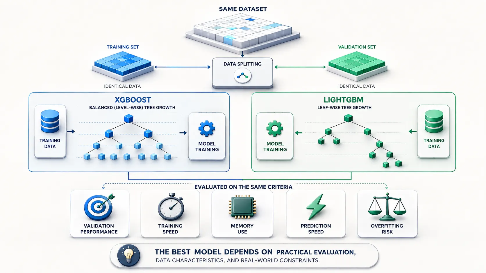
The practical approach is to build a simple baseline with both models using the same training and validation split.
Compare:
Validation performance
Training time
Memory use
Prediction speed
Overfitting difference
Then choose the model that solves the real problem—not the one that sounds more advanced.
The central difference should now feel clear:
XGBoost usually gives you a controlled and highly configurable boosting system.
LightGBM is built around fast histogram learning and leaf-wise growth.
The next question is not:
“Which library is more famous?”
The better question is:
“Which library fits my dataset, resources, and prediction goal?”
Important Parameters You Should Understand Before Tuning
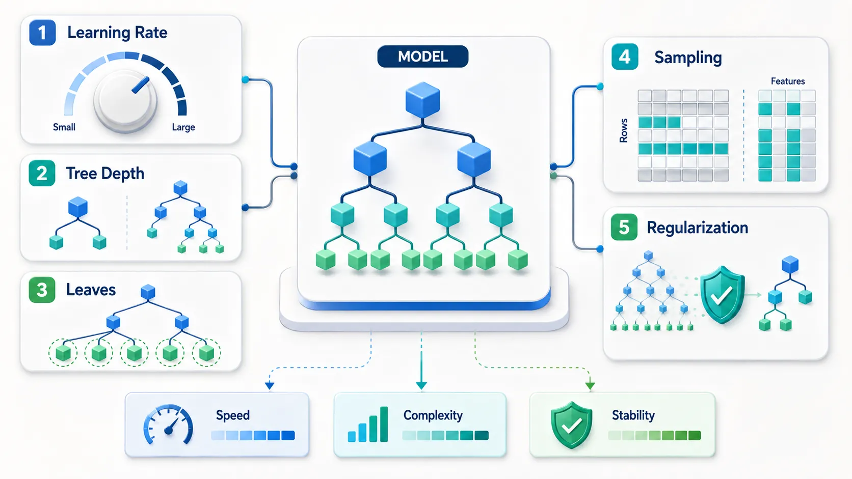
You do not need to change every setting on the first day. Start with the few parameters that control how fast the model learns and how complex its trees become.
Learning Rate
The learning rate controls how much influence each new tree has on the final prediction.
A high learning rate makes larger corrections and may need fewer trees. It can also move too quickly. A lower learning rate makes smaller corrections and usually needs more boosting rounds.
The useful lesson is not “always use a small value.” Tune the learning rate together with the number of trees because these settings work as a pair. Both XGBoost and LightGBM documentation treat the learning rate and boosting rounds as closely connected tuning decisions.
Tree Complexity
In XGBoost, max_depth is a major control for tree complexity. Deeper trees can capture detailed relationships, but they also use more memory and may overfit.
In LightGBM, num_leaves needs special attention because the model grows leaf-wise. More leaves allow it to create more detailed rules. Its official tuning guide recommends controlling num_leaves, max_depth, and the minimum data allowed in a leaf when overfitting appears.
Imagine a rule saying:
“Customers from one city, using one device, booking one hotel type at a particular hour, will cancel.”
If only two customers match it, the rule may be an accident rather than a useful pattern.
Increasing the minimum data required in a leaf can stop the model from creating such narrow rules. This parameter is commonly called min_data_in_leaf in LightGBM, while XGBoost offers related complexity controls such as min_child_weight.
Row and Feature Sampling
XGBoost uses settings such as subsample and colsample_bytree. LightGBM offers similar controls through parameters such as bagging_fraction and feature_fraction.
These settings let each tree learn from only part of the rows or columns. This can reduce overfitting because every tree does not depend on exactly the same information.
Sampling may also improve training speed, but removing too much information can weaken the model.
How to Control Overfitting
A common warning sign is a large gap between training and validation performance.
Suppose a hotel cancellation model reaches 98% accuracy on training data but only 78% on validation data. It has probably learned the training records too closely.
You can respond by:
Using less complex trees
Reducing the number of leaves
Increasing the minimum data per leaf
Sampling rows or features
Adding regularization
Lowering the learning rate
Early stopping is another practical safeguard.
Allow the model to train for a generous number of rounds and check its performance on validation data after each round. When the selected metric stops improving for a chosen number of rounds, training ends.
Both XGBoost and LightGBM support early stopping when validation data and an evaluation metric are provided.
It is like preparing for an exam. Practice helps, but continuing after your performance has stopped improving may add tiredness rather than useful learning.
Choose the Right Evaluation Metric
Accuracy is not always the right score.
Imagine that only 3 out of every 100 online transactions are fraudulent. A model that predicts “not fraud” every time would be 97% accurate, yet it would fail at its real job.
For an imbalanced classification problem, precision, recall, F1 score, or an area-under-the-curve metric may be more useful.
For predicting a number, such as hotel price or delivery time, MAE or RMSE may be suitable. These metrics measure different kinds of prediction error, so the right choice depends on what mistakes matter most in the actual project.
The evaluation metric should reflect the cost of a wrong decision.
If missing a fraudulent payment is more dangerous than checking a safe payment manually, recall may deserve more attention.
If falsely blocking genuine customers is expensive, precision also matters.
Compare XGBoost and LightGBM with the same validation method and the same business-focused metric—not training accuracy alone.
Common Mistakes Beginners Should Avoid
Tuning Before Creating a Baseline
Begin with sensible settings and record the result.
After that, change a small group of parameters and check whether the validation result actually improves. Changing ten settings together makes it difficult to understand which change helped.
Repeatedly Checking the Test Set
Use training and validation data for model selection. Keep the test set separate for an honest final check.
When the test set repeatedly influences model decisions, it slowly stops behaving like unseen data.
Allowing Data Leakage
Data leakage happens when the model receives information that would not be available at prediction time.
For example, a hotel cancellation model must not use a field created only after the booking has already been cancelled.
The validation score may look excellent, but the model will fail in a live system because that information will not exist when the prediction is needed.
Scikit-learn’s official guidance warns that leakage creates overly optimistic evaluation results and weaker performance on genuinely new data.
Assuming Faster Always Means Better
Training speed matters, but it is not the only requirement.
Prediction time, memory consumption, stability, explainability, deployment cost, and future maintenance also matter in a production system.
XGBoost or LightGBM: Which One Should You Choose?
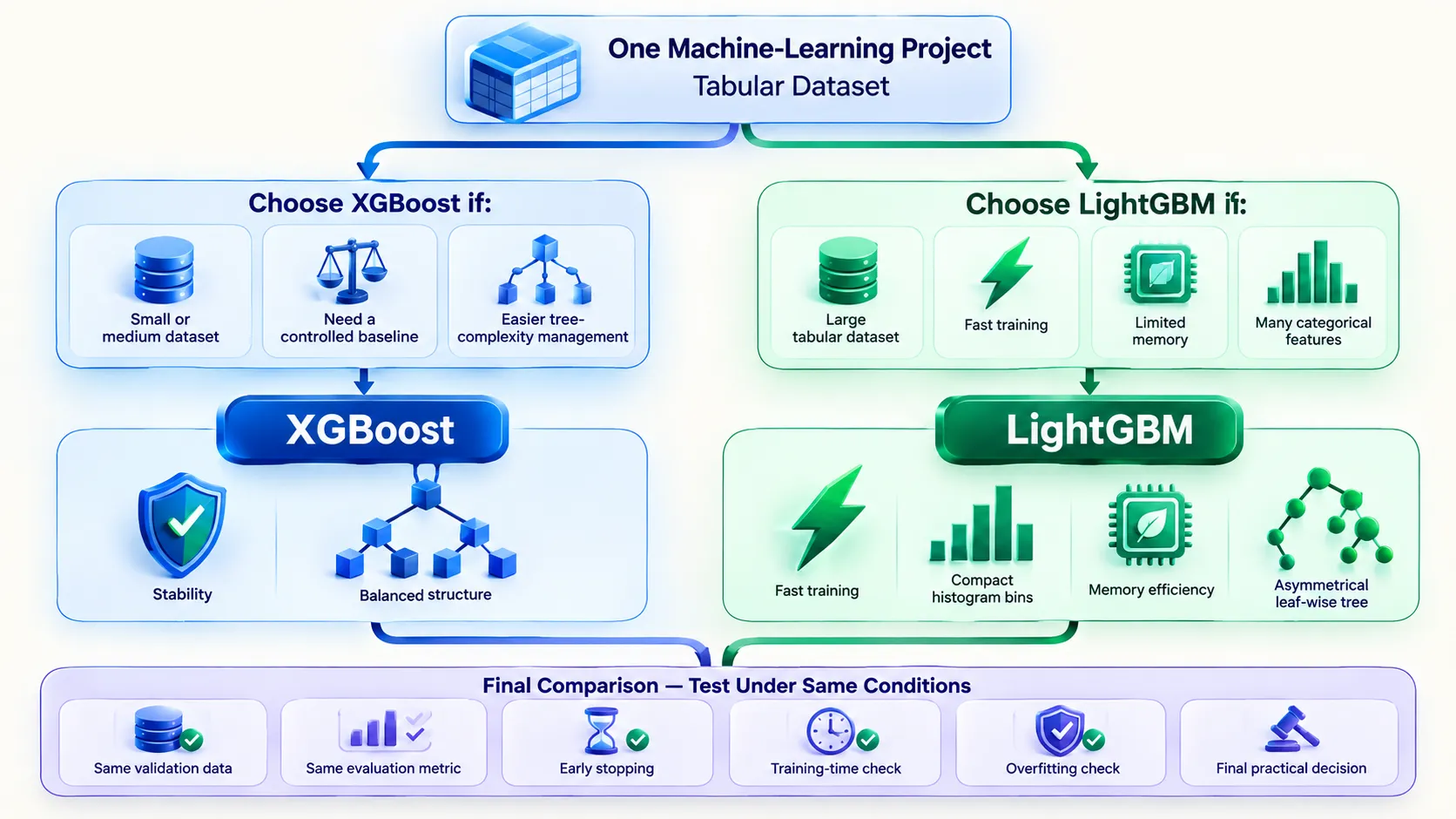
Choose XGBoost as your first experiment when you want a controlled baseline, your dataset is small or medium-sized, or you find depth-based tree limits easier to understand.
Choose LightGBM when you are working with a large tabular dataset, training time or memory is a major concern, or the data contains many useful categorical features.
Watch leaf complexity carefully when using LightGBM on a smaller dataset.
These are practical starting directions, not permanent rules. The final result still depends on your data, feature quality, validation method, parameters, and hardware.
A reliable workflow is simple:
Train both models on the same data split.
Use the same evaluation metric.
Apply early stopping.
Record validation performance.
Compare training and prediction time.
Check memory use and overfitting.
Select the model that gives the best practical balance.
Final Thoughts
The XGBoost vs LightGBM comparison has no universal winner because machine-learning problems are not identical.
XGBoost often feels controlled and dependable.
LightGBM often feels fast and flexible.
Both can produce excellent results, and both can overfit when used carelessly.
The real skill is not memorizing which library is “best.” It is understanding how gradient boosting learns, choosing meaningful features, preventing leakage, validating honestly, and matching the evaluation metric to the real problem.
Once you can do that, choosing between XGBoost and LightGBM becomes much easier.
You are no longer selecting a model because it is popular.
You are selecting it because you understand what your data and your project actually need.


