


The Real Problem Is Not Data
Modern companies rarely suffer from a lack of data.
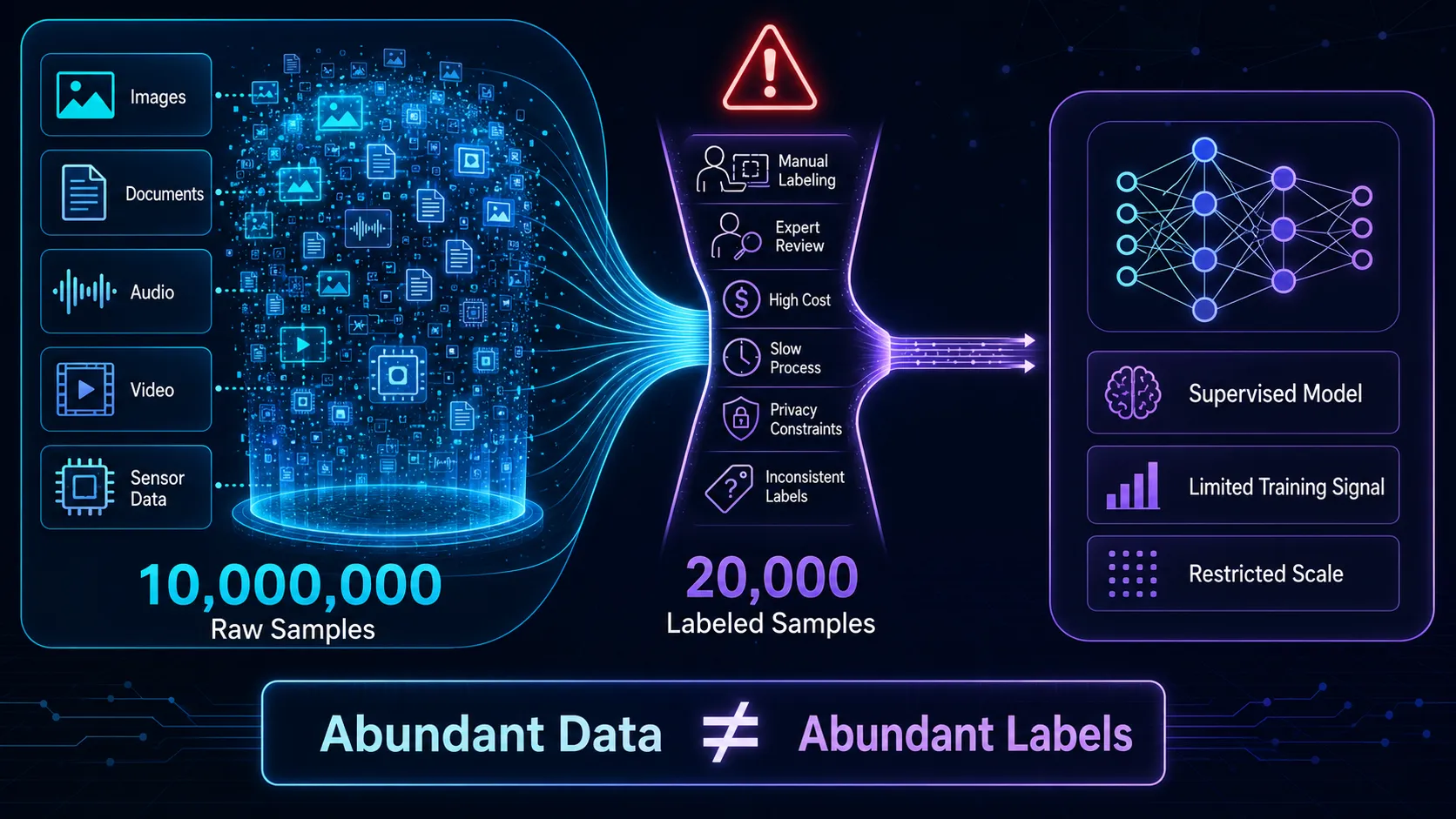
They store millions of images, documents, audio files, videos, medical scans, transaction records, and sensor streams. Most of that data never reaches a machine learning model.
The reason is simple.
Nobody labeled it.
A computer vision team may own ten million factory images but only twenty thousand defect annotations. A hospital may store years of scans, while specialist labels exist for only a small fraction.
The same problem appears in language systems.
Companies archive support tickets, contracts, product descriptions, and internal documents. Yet few teams can afford to classify every sentence by topic, intent, urgency, sentiment, or meaning.
Raw data grows quickly.
Human annotation does not.
This gap creates one of the most expensive constraints in machine learning: the label bottleneck.
Why Manual Labeling Fails at Scale
Supervised learning relies on labeled examples.
A model receives an input, predicts an answer, compares that answer with a human-provided target, and adjusts its parameters.
That process works well when labels remain cheap and clear.
Many real projects meet neither condition.
A person can label a photograph as “shoe” within seconds. That same person cannot reliably mark a rare neurological pattern in a brain scan.
Specialized datasets require specialists.
Radiologists label medical scans. Lawyers classify legal clauses. Engineers identify industrial faults. Native speakers review low-resource languages.
Their time costs money.
Their availability also limits scale.
Annotation quality creates another problem. Two experts may interpret the same example differently, especially when categories overlap or instructions leave room for judgment.
Even simple labels can drift.
One reviewer marks an image as “sportswear.” Another selects “footwear.” A third chooses “running shoe.”
The dataset now contains inconsistency before training even starts.
Privacy adds another barrier.
Organizations cannot freely send medical records, financial documents, private messages, or confidential business files to large external labeling teams.
The data exists.
The labels do not.
What Is Self-Supervised Learning?
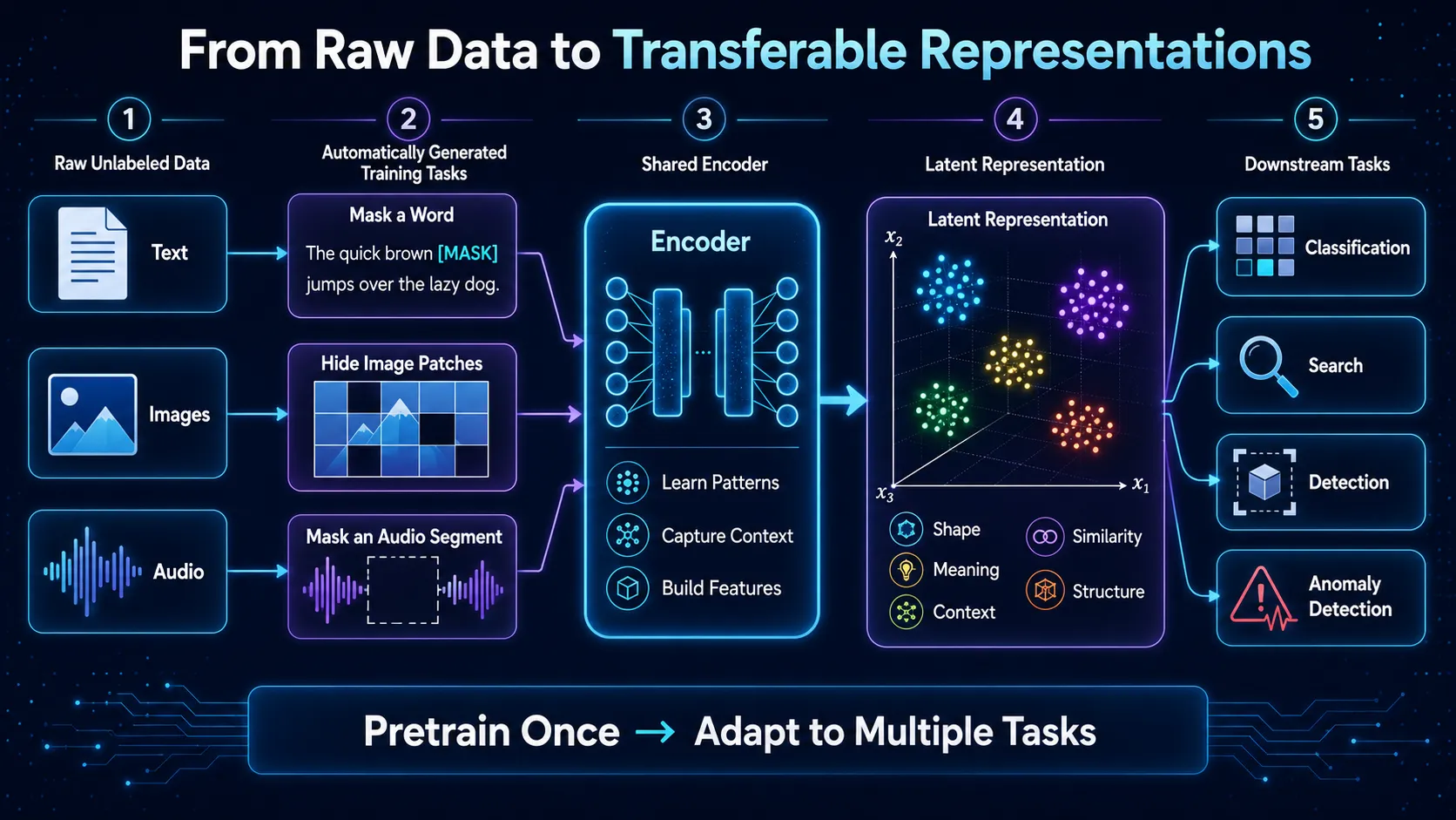
Self-supervised learning trains a model with targets created from the raw data itself.
Instead of asking a human to label every sample, engineers design a task where one part of the data predicts another part.
A language model may predict a hidden word.
An image model may reconstruct missing patches.
An audio model may recover a masked sound segment.
A video model may predict what happens next.
The original data supplies the answer.
That detail separates self-supervision from ordinary manual annotation.
Core idea: Self-supervised learning does not remove supervision. It changes where the supervision comes from.
The model still needs a training target.
It still calculates an error.
It still updates its parameters.
But a human does not write the target by hand.
This explains the phrase self-supervised learning without labeled data. The model learns from unlabeled raw material, while the training pipeline automatically generates a temporary target.
How Data Creates Its Own Training Task
Take a complete sentence:
The engineer deployed the model to production.
The training pipeline hides one word:
The engineer deployed the model to [MASK].
The original sentence already contains the correct target:
Target: production
No annotator needs to create a separate answer sheet.
The system takes an existing piece of text, removes a meaningful part, and asks the model to recover it.
The same logic works with images.
A training pipeline divides an image into patches, hides several patches, and asks the model to reconstruct the missing regions.
It can also create two different crops from one photograph.
The crops may look different, but they still come from the same source image. The model learns to connect their underlying meaning.
Audio systems follow similar patterns.
They mask a short section of speech and train the model to identify or reconstruct the missing acoustic content.
These tasks generate supervision at scale.
One raw dataset can produce millions of training problems without millions of manual labels.
The Role of the Pretext Task
Researchers call the automatically created training problem a pretext task.
The model solves this temporary task to learn patterns that will help with a later business or research task.
The pretext task does not need to match the final objective.
A company may want to detect damaged products. During pretraining, the model may reconstruct missing image regions rather than classify defects.
Why use an indirect task?
Because reconstruction forces the model to study shape, texture, edges, position, and object structure.
Those features can later support defect detection.
Common self-supervised learning pretext task examples include:
Predicting masked words
Reconstructing hidden image patches
Matching two views of the same sample
Predicting future video frames
Recovering missing audio segments
Reordering shuffled sequence elements
A useful pretext task makes the model learn information that transfers.
A weak one teaches shortcuts.
From Raw Input to Training Signal
Traditional supervised learning usually follows this structure:
Input + Human Label → Model → Prediction → Error
Self-supervised learning changes the source of the target:
Raw Data → Automatic Transformation → Generated Target
For text:
Complete Sentence → Mask Word → Predict Original Word
For images:
Complete Image → Hide Patches → Reconstruct Missing Patches
For contrastive learning:
One Image → Create Two Views → Learn That Both Views Belong Together
The model still learns through an objective function.
The objective measures the distance between the prediction and the generated target.
The training process then updates the model so that future predictions improve.
The engineering challenge moves upstream.
Teams must design transformations that preserve useful meaning while creating a difficult enough learning task.
What the Model Actually Learns
The model does not only learn how to fill blanks.
It learns representations.
A representation converts an input into a structured set of numbers. Those numbers capture patterns that the model considers useful.
An image representation may encode shape, texture, boundaries, object parts, and spatial relationships.
A text representation may encode meaning, context, syntax, topic, and relationships between words.
An audio representation may capture rhythm, pronunciation, speaker traits, and acoustic structure.
Strong representations make later tasks easier.
When similar products receive similar representations, a small classifier can separate shoes, bags, and watches with fewer labeled examples.
When related sentences appear close together in the representation space, a search engine can retrieve relevant content even when the wording differs.
This process drives representation learning.
The model first learns general structure from a large raw dataset. Engineers then adapt that knowledge to a smaller, task-specific dataset.
Self-Supervised Learning vs Unsupervised Learning
People often treat self-supervised learning and unsupervised learning as identical.
They overlap, but they do not follow the same training logic.
Unsupervised learning searches for structure without human-provided targets. Clustering provides a common example.
A clustering algorithm groups similar customers, documents, or products without receiving a correct category for each sample.
Self-supervised learning creates an explicit prediction problem.
The system may ask:
Which token is missing?
Which patch belongs in this region?
Do these two views come from the same source?
What event follows this sequence?
Which audio segment fits this context?
The model receives a generated target and optimizes against it.
That structured objective gives engineers tighter control over what the model learns.
What Self-Supervised Learning Does Not Do
Self-supervised learning does not remove human decisions.
Engineers still choose the dataset, architecture, transformations, loss function, and evaluation method.
The method also does not guarantee useful knowledge.
A model learns whatever the training objective rewards.
If an image pipeline removes medically meaningful color, the model may learn to ignore a feature that doctors need.
If a contrastive system treats two similar samples as unrelated, it may push useful representations apart.
If the task feels too easy, the model may rely on surface-level clues.
Self-supervision also does not eliminate labeled data from every stage.
Teams still need labels for fine-tuning, testing, safety validation, benchmarking, and production monitoring.
The advantage comes from label efficiency.
A model can learn broad patterns from millions of unlabeled examples, then adapt to a specific task with a much smaller labeled dataset.
Why Self-Supervised Learning Matters
Self-supervised learning changes the value of raw data.
Unlabeled files no longer represent unfinished annotation work. They become training material.
This matters most in fields where data grows faster than expert labeling capacity.
Medical imaging, robotics, speech recognition, cybersecurity, industrial inspection, search, and document intelligence all face that pressure.
The method also supports reuse.
Teams can pretrain one encoder on broad data, then adapt it for classification, retrieval, detection, segmentation, forecasting, or anomaly detection.
That does not make the process cheap or automatic.
Large-scale pretraining may require serious compute, careful data governance, strong evaluation, and disciplined engineering.
But it addresses a hard practical question:
How can a model learn from the enormous volume of information that humans will never have time to label?
How Self-Supervised Learning Works
The Two-Stage Training Strategy
Self-supervised learning usually separates training into two stages.
First, the model learns general patterns from a large unlabeled dataset. Then, engineers adapt the pretrained model to a specific downstream task.
The first stage builds reusable representations.
The second stage turns those representations into practical outputs such as classifications, detections, search results, transcriptions, or forecasts.
This separation gives self-supervised learning much of its value.
A team can pretrain one encoder on millions of raw examples, then reuse it across several smaller labeled tasks.
How Does Self-Supervised Learning Work Step by Step?
The exact architecture changes across text, vision, audio, and video.
The core workflow stays remarkably consistent.
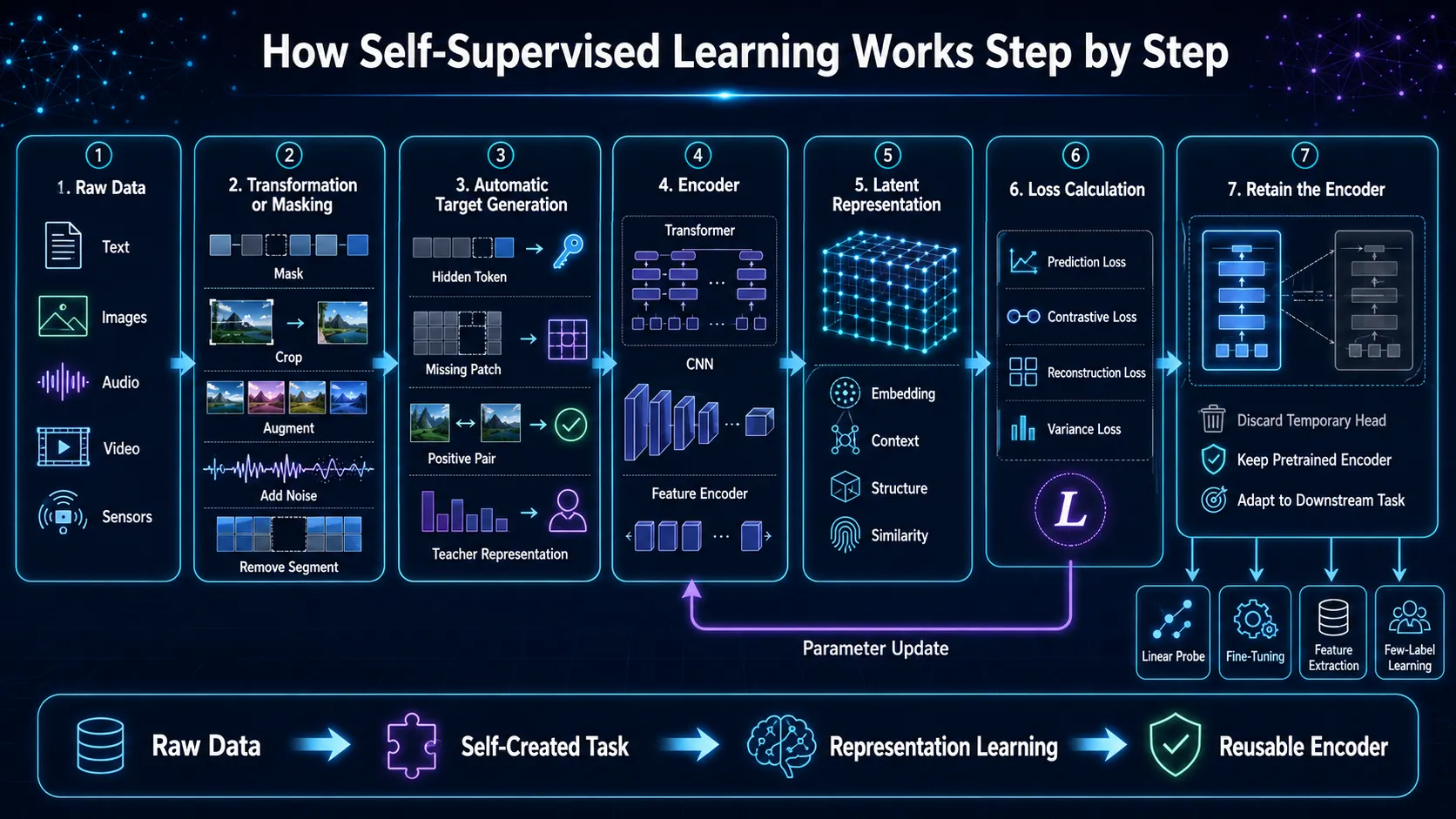
Step 1: Collect Raw Data
The pipeline begins with unlabeled data.
That data may include documents, images, speech recordings, videos, medical scans, transaction sequences, or industrial sensor readings.
At this stage, the samples do not need human-written categories.
They only need enough internal structure for the model to learn useful relationships.
A language dataset contains relationships between words.
An image contains relationships between patches, shapes, textures, and objects.
An audio recording contains relationships between sounds across time.
Step 2: Apply a Transformation or Mask
The training pipeline modifies each sample.
It may hide part of the input, create multiple views, add controlled noise, crop an image, shuffle a sequence, or remove a time segment.
The transformation creates the learning problem.
For masked language training:
Original: The model detected a damaged component.
Input: The model detected a [MASK] component.
For image training:
Original Image → Divide Into Patches → Hide Selected Patches
For contrastive training:
One Image → Random Crop A → Random Crop B
Both crops come from the same source, so the pipeline treats them as related views.
Step 3: Generate the Training Target
The pipeline extracts the target from the original sample.
For masked text, the hidden word becomes the target. For masked images, the original pixel patches become the reconstruction target.
Contrastive methods use relationships instead of missing content.
Two transformed views from the same sample create a positive pair. Views from different samples often create negative pairs.
Teacher-student methods create another kind of target.
A slowly updated target network produces a representation, and the online network learns to predict it.
No human writes these targets.
The pipeline generates them automatically.
Step 4: Build a Latent Representation
The encoder processes the transformed input.
It converts raw data into a compact numerical representation called an embedding or latent representation.
Mathematically:
h = fθ(x)
Here, x represents the transformed input, fθ represents the encoder, and h represents the learned embedding.
The encoder may use a Transformer, convolutional neural network, vision transformer, recurrent network, or another architecture.
Its job remains the same: capture useful structure.
A good representation keeps meaningful information while discarding noise that does not help later tasks.
Step 5: Process the Representation
Many SSL systems add a temporary component after the encoder.
This component may act as a projection head, prediction head, decoder, quantizer, or target network.
For example:
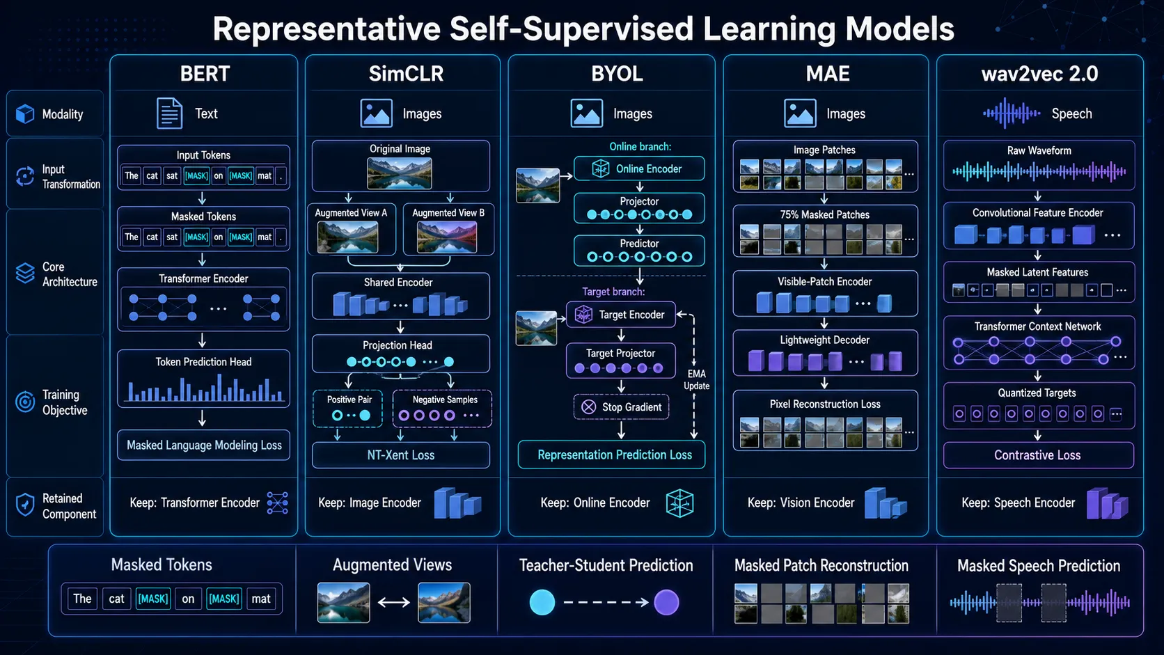
SimCLR uses a projection head.
BYOL adds a projector and predictor.
MAE uses a reconstruction decoder.
wav2vec 2.0 uses a quantization module.
BERT uses a token prediction head.
These components shape the pretraining objective.
Engineers often remove them after pretraining.
Step 6: Calculate the Loss
The loss function measures how well the model solves the self-created task.
A masked language model may use cross-entropy loss to compare predicted tokens with original tokens.
An image reconstruction model may measure the difference between predicted pixels and hidden pixels.
A contrastive model compares similarities:
High similarity for positive pairs
Low similarity for negative pairs
The optimizer uses the loss to update the model parameters.
Each update should move the representation toward the properties that the training objective rewards.
Step 7: Retain the Encoder
After pretraining, engineers usually keep the encoder.
They discard temporary components such as reconstruction decoders or projection heads unless the downstream task still needs them.
The retained encoder now acts as a feature extractor.
A team can freeze it, partially update it, or fine-tune the entire network with labeled data.
That completes the basic workflow:
Raw Data
→ Transformation or Masking
→ Automatic Target Generation
→ Encoder
→ Latent Representation
→ Loss Calculation
→ Retained Encoder
→ Downstream Task
Four Major Self-Supervised Objective Families
Different SSL methods create different training problems.
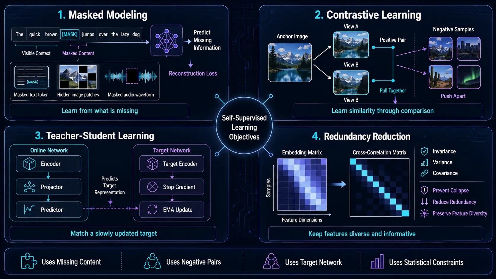
Most widely used architectures fall into four broad objective families.
1. Masked Modeling
Masked modeling removes part of the input and asks the model to recover it.
The visible content provides context. The hidden content provides the target.
Text models often mask tokens:
Input: The server returned an unexpected [MASK].
Target: error
Vision models may hide image patches:
Visible Patches → Encoder → Decoder → Reconstructed Patches
Audio models can mask spans of latent speech features.
The model must infer the missing signal from the surrounding context.
Masked modeling works well when the input contains strong internal dependencies.
Words depend on nearby words. Image regions depend on neighbouring shapes. Speech segments depend on earlier and later sounds.
The loss usually compares the prediction with the original hidden content.
Token-based systems often use cross-entropy loss. Pixel-based systems may use mean squared error or a related reconstruction objective.
Masked modeling can learn rich contextual representations.
However, the masking strategy matters. Easy masks may teach trivial shortcuts, while destructive masks may remove too much useful context.
2. Contrastive Learning
Contrastive learning trains the model to compare examples.
It pulls related representations closer and pushes unrelated representations apart.
A typical image pipeline creates two augmented views from the same image.
Those views form a positive pair.
Views from different images act as negative pairs.
The model encodes both views:
z₁ = g(f(x₁))
z₂ = g(f(x₂))
The encoder f creates representations, while the projection head g maps them into a space designed for the contrastive loss.
Objectives such as InfoNCE or NT-Xent reward high similarity between positive pairs.
They penalize high similarity between negative pairs.
Data augmentation plays a central role.
If augmentations remain too weak, the model may memorize superficial details. If they become too aggressive, they may change the sample’s meaning.
Contrastive learning also depends on negative-sample quality.
Two different images may belong to the same semantic class. Treating them as negatives can push useful representations apart.
3. Non-Contrastive Teacher-Student Learning
Non-contrastive methods remove explicit negative pairs.
They train one network to predict the representation produced by another network.
The online network learns through gradient updates.
The target network changes more slowly, often through an exponential moving average of the online network’s parameters.
A simplified flow looks like this:
View A → Online Encoder → Projector → Predictor
View B → Target Encoder → Target Projection
The loss encourages the online prediction to match the target representation.
A stop-gradient operation prevents the target branch from updating through the same loss path.
This design creates an asymmetric learning process.
That asymmetry, combined with the predictor, target updates, and normalization, helps the model avoid mapping every input to the same representation.
Non-contrastive learning often simplifies batch construction because it does not require large sets of explicit negatives.
It still requires careful architecture and training stability.
4. Redundancy Reduction and Variance Regularization
These methods focus directly on the statistical properties of learned features.
They encourage two views of the same sample to produce similar representations while preventing every feature dimension from carrying identical information.
Barlow Twins uses a cross-correlation matrix between two representation batches.
It pushes the diagonal values toward one and the off-diagonal values toward zero.
The diagonal objective encourages invariance.
The off-diagonal objective reduces redundancy.
VICReg separates the problem into three terms:
Invariance: Keep paired representations close.
Variance: Maintain enough variation across each feature dimension.
Covariance: Reduce duplication between dimensions.
The variance term helps prevent collapse.
The covariance term encourages different dimensions to capture different information.
These methods do not rely on explicit negative pairs.
They control representation quality through variance, correlation, and feature diversity.
Contrastive vs Non-Contrastive Self-Supervised Learning
The main difference lies in how each method avoids trivial representations.
Contrastive learning compares positive and negative samples. It prevents collapse by forcing different samples apart.
Non-contrastive learning removes explicit negatives.
It relies on architectural asymmetry, stop-gradient operations, target networks, predictors, normalization, or variance-based constraints.
Neither family wins every task.
Dataset size, batch size, augmentation quality, compute limits, and downstream requirements should drive the choice.
Representative Model Walkthroughs
BERT: Masked Language Modeling
BERT uses an encoder-only Transformer.
The training pipeline masks selected tokens and asks the model to predict the original words from surrounding context.
Each token attends to words on both sides.
This bidirectional context helps BERT learn syntax, meaning, word relationships, and sentence structure.
The token prediction head supports pretraining.
Afterward, engineers retain the Transformer encoder and add a task-specific head for classification, extraction, or question answering.
SimCLR: Contrastive Visual Learning
SimCLR creates two augmented views from each image.
A shared encoder, commonly a ResNet in the original design, converts both views into representations.
A multilayer projection head maps those representations into a contrastive space.
The NT-Xent loss pulls matching views together and pushes other samples apart.
After pretraining, engineers discard the projection head.
They retain the encoder for image classification or other vision tasks.
BYOL: Learning Without Explicit Negatives
BYOL uses two networks.
The online network contains an encoder, projector, and predictor. The target network contains an encoder and projector.
Two augmentations of one image enter separate branches.
The online network predicts the target network’s representation.
An exponential moving average updates the target network.
The stop-gradient operation blocks direct optimization through the target branch.
After training, engineers retain the online encoder.
MAE: Masked Image Reconstruction
Masked Autoencoders divide an image into fixed-size patches.
The pipeline hides a large percentage of those patches, often around 75 percent.
The encoder processes only the visible patches.
A lightweight decoder receives the encoded visible patches plus mask tokens and reconstructs the missing pixels.
This asymmetric design reduces encoder computation during pretraining.
After training, engineers remove the decoder and retain the visual encoder.
wav2vec 2.0: Learning from Raw Speech
wav2vec 2.0 begins with raw audio.
A convolutional feature encoder converts the waveform into latent speech representations.
The pipeline masks spans within that latent sequence.
A Transformer context network processes the masked sequence.
A quantization module creates discrete target representations from the original unmasked features.
The contrastive loss asks the model to identify the correct quantized target among distractors.
Engineers then fine-tune the pretrained network with transcribed speech for automatic speech recognition.
Choosing, Applying, and Evaluating Self-Supervised Learning
A self-supervised model can achieve a low pretraining loss and still fail on the task that matters.
Engineering teams must compare learning paradigms, select the right objective, test transfer quality, and inspect the representation itself.
Self-Supervised vs Other Learning Paradigms
The main difference between learning paradigms lies in the source of the training signal.
The following responsive table compares supervised, unsupervised, semi-supervised, and self-supervised learning.
The self-supervised vs unsupervised learning distinction often causes confusion.
Unsupervised methods search for structure without a defined prediction target. Self-supervised systems construct an explicit target and optimize a measurable objective against it.
Major SSL Methods Compared
Each SSL method encodes a different assumption about useful information.
BERT trusts contextual language prediction. SimCLR trusts view invariance. MAE trusts reconstruction. BYOL trusts teacher-student consistency.
No method wins by default.
The right choice depends on modality, dataset scale, hardware limits, augmentation validity, and the final deployment task.
Engineering Decision Framework
Method selection should begin with the structure of the data.
Ask what information can be hidden, transformed, compared, or predicted without destroying the meaning required downstream.
Step 1: Identify the Modality
For text, masked-token prediction remains a strong starting point because language contains dense contextual dependencies.
For images, teams often choose between masked reconstruction, contrastive learning, and non-contrastive view matching.
For speech, temporal masking and contextual prediction usually fit the signal better than image-style spatial cropping.
For video and sensors, sequence order, temporal continuity, and future-state prediction carry valuable supervision.
Step 2: Check Whether Safe Augmentations Exist
Contrastive and teacher-student methods depend heavily on augmentations.
An augmentation should alter surface details while preserving the semantic identity needed by the downstream task.
Random cropping may work for consumer photographs.
The same crop could remove a tiny tumour, manufacturing crack, or safety-critical object from a specialized image.
When augmentations risk changing the label, masked modeling may provide a safer objective.
Step 3: Match the Method to Dataset Size
Small datasets create a narrow learning signal.
A high-capacity model may memorize transformations rather than learn general patterns.
Masked modeling often works when each sample contains rich internal structure. Contrastive learning benefits from varied samples and diverse positive views.
Very large datasets support stronger pretraining.
They also increase storage, data-cleaning, duplication, and distribution-shift concerns.
Step 4: Match the Method to Compute Budget
Contrastive methods may require large batches or memory queues to provide enough negative examples.
That increases accelerator memory and communication costs.
BYOL-style methods remove explicit negatives, but they maintain multiple network branches and require stable optimization.
MAE reduces encoder workload by processing only visible patches, which can make high masking ratios computationally attractive.
Step 5: Start From the Downstream Task
Classification may benefit from globally separated embeddings.
Detection and segmentation need spatial detail.
Retrieval systems need meaningful similarity geometry, while forecasting systems need temporal structure and causal continuity.
Use this compact decision tree:
Does the input contain predictable missing structure?
├── Yes
│ ├── Text, images, audio → Masked modeling
│ └── Sequential data → Temporal prediction
└── No
└── Can safe semantic-preserving views be created?
├── Yes
│ ├── Reliable negatives available → Contrastive learning
│ └── Negatives unreliable or expensive → Teacher-student or variance-based SSL
└── No
└── Reassess the data, objective, or need for self-supervised pretraining
Real-World Applications by Modality
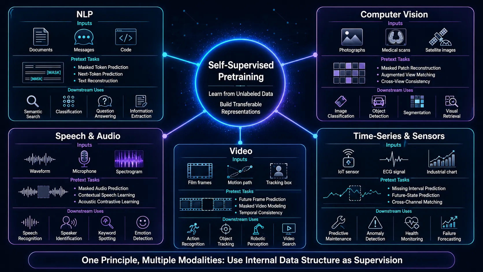
Natural Language Processing
Language models learn from masked tokens, next-token prediction, sentence relationships, or corrupted text reconstruction.
Teams reuse those representations for semantic search, document classification, entity extraction, question answering, moderation, and domain-specific assistants.
Computer Vision
Vision systems learn through masked patches, augmented image pairs, temporal frames, or cross-view consistency.
Common uses include medical imaging, industrial inspection, satellite analysis, product search, object detection, and semantic segmentation.
Speech and Audio
Audio models learn phonetic, acoustic, speaker, and contextual features from raw waveforms or latent sequences.
They support speech recognition, speaker identification, emotion detection, keyword spotting, and low-resource language systems.
Video
Video provides spatial and temporal supervision at the same time.
Models can predict future frames, match clips from the same sequence, track objects across time, or reconstruct masked video tokens.
Applications include action recognition, robotic perception, content indexing, surveillance analysis, and autonomous navigation.
Time-Series and Sensors
Sensor systems can predict missing intervals, future values, transformed views, or relationships between channels.
Teams use these representations for predictive maintenance, anomaly detection, health monitoring, fraud detection, and equipment-failure forecasting.
How to Evaluate Self-Supervised Learning Models
Pretraining loss measures performance on the pretext task.
It does not prove downstream value.
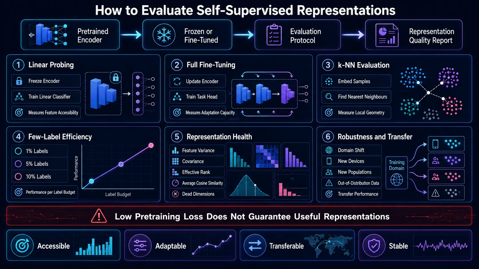
A proper evaluation should measure accessibility, adaptability, label efficiency, robustness, and representation health.
Linear Probing vs Full Fine-Tuning
Linear probing freezes the pretrained encoder.
Engineers train only a linear classifier on top of the fixed representation.
Strong linear-probe results show that the encoder already organizes useful features in a directly accessible form.
The test remains narrow.
A weak linear probe does not always mean the representation lacks useful information.
Full fine-tuning updates both the encoder and the task head.
This protocol measures how well the pretrained model adapts when labeled data can reshape its internal features.
The comparison between linear probing vs fine-tuning self-supervised learning reveals two different qualities.
Linear probing tests feature accessibility. Fine-tuning tests adaptation capacity.
A reliable benchmark should report both.
k-NN Evaluation
k-nearest-neighbour evaluation requires no learned classifier head.
The system embeds each labeled example, finds nearby representations, and predicts from the labels of the closest neighbours.
This test offers a fast check of embedding geometry.
If semantically similar samples cluster together, k-NN accuracy should rise.
Poor k-NN performance may expose weak local structure even when full fine-tuning performs well.
Few-Label Efficiency
Few-label evaluation measures performance using a small fraction of labeled data.
Common splits include 1%, 5%, 10%, or a fixed number of examples per class.
This protocol tests the central promise of SSL: reducing dependence on manual labels.
A useful pretrained model should outperform random initialization when both systems receive the same limited labeled set.
Representation Health Metrics
Downstream accuracy cannot expose every representation failure.
Engineers should inspect the embeddings directly.
Feature variance measures whether each embedding dimension changes across samples.
Near-zero variance across many dimensions signals collapse or inactive features.
Covariance measures whether dimensions carry duplicate information.
Large off-diagonal covariance values suggest that several dimensions encode nearly identical patterns.
Effective rank estimates how many meaningful directions the representation uses.
A low effective rank can indicate dimensional collapse even when the embedding vector contains hundreds of fields.
Other warning signs include:
Nearly identical embeddings across unrelated samples
Extremely high average cosine similarity
Dead or constant feature dimensions
Poor class separation
Unstable feature statistics across batches
Sharp degradation under domain shift
A healthy representation should preserve useful variation, suppress irrelevant noise, transfer with limited labels, and remain stable outside the pretraining distribution.
A practical evaluation report should combine linear probing, full fine-tuning, k-NN testing, few-label performance, robustness tests, and feature-statistics analysis.
No single metric tells the whole story.
Failure Modes, Edge Cases, and Practical Takeaways
Self-supervised learning can extract strong representations from raw data.
It can also learn useless shortcuts, collapse into nearly identical embeddings, or consume more compute than the downstream value justifies.
The pretraining objective controls what the model preserves.
That makes objective design, data validation, and evaluation just as important as model architecture.
Common Failure Modes in Self-Supervised Learning
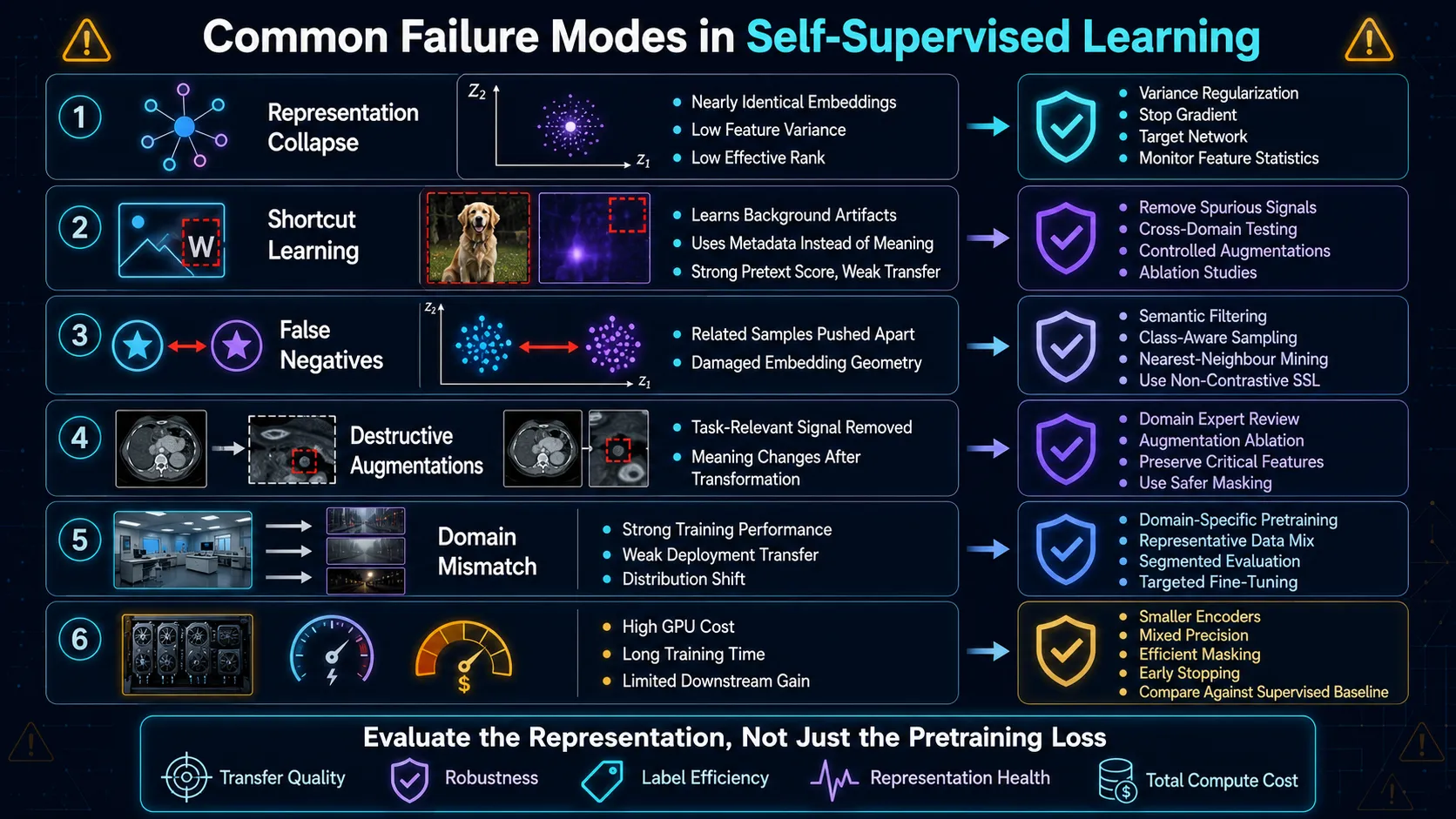
Representation Collapse
Representation collapse occurs when the encoder maps different inputs to identical or nearly identical embeddings.
The model technically minimizes its training loss, but the representation carries little information about the input.
This risk appears most clearly in non-contrastive architectures.
Without negative samples or explicit variance controls, the model may discover that producing the same output for every example creates an easy solution.
Engineers can monitor feature variance, embedding similarity, covariance, and effective rank during training.
Stop-gradient operations, target networks, predictor asymmetry, normalization, and variance regularization can reduce collapse risk.
A healthy representation should change meaningfully across different samples.
If most feature dimensions remain constant, stop training and inspect the objective before spending more compute.
Shortcut Learning
A model may solve the pretext task without learning the semantic information needed downstream.
It finds the easiest available signal.
An image model might identify camera artifacts instead of objects. An audio model might rely on recording equipment rather than speech content.
A medical model may associate hospital-specific markers with disease labels.
These shortcuts often produce strong pretraining metrics and weak deployment performance.
Test the encoder across different devices, locations, time periods, and data sources.
Remove suspicious metadata, balance collection environments, and use augmentations that block known shortcuts without destroying valid information.
False Negatives
Contrastive learning often treats samples from different records as negative pairs.
That assumption can fail.
Two photographs may show the same product category. Two audio clips may contain the same speaker. Two medical scans may share the same pathology.
Pushing these related examples apart damages the representation space.
This problem becomes severe when the dataset contains many semantically similar samples.
Use larger semantic groupings, nearest-neighbour filtering, class-aware sampling when limited labels exist, or non-contrastive methods when reliable negatives remain difficult to define.
Destructive Augmentations
Augmentations should change surface appearance while preserving task-relevant meaning.
That boundary depends on the domain.
Cropping a consumer photograph may preserve the main object.
The same crop may remove a tiny manufacturing crack, traffic sign, tumour, or safety event.
Colour distortion may help general object recognition but erase clinically meaningful tissue differences.
Validate every augmentation against the downstream task.
Run controlled ablation tests and compare performance with and without each transformation.
Domain experts should review augmentation policies in medical, industrial, financial, and safety-critical systems.
Domain Mismatch
Pretraining helps most when the raw data resembles the deployment environment.
Large datasets do not guarantee relevant representations.
A speech model trained on clean studio recordings may struggle with factory noise.
A vision encoder trained on internet photographs may miss patterns in thermal images or satellite data.
Measure transfer across real deployment segments.
Fine-tune on domain-specific samples, mix representative data into pretraining, and track performance separately for each device, region, population, or operating condition.
Compute Inefficiency
Self-supervised pretraining can reduce labeling costs while increasing infrastructure costs.
Large models may require long training runs, high-memory accelerators, distributed systems, and substantial energy.
More pretraining does not always create better business outcomes.
A smaller supervised model may outperform a large SSL pipeline when labels remain affordable and the task stays narrow.
Compare total costs.
Include annotation, storage, preprocessing, hardware, experimentation, monitoring, and retraining.
Use smaller encoders, mixed precision, efficient masking, early stopping, and frozen-feature baselines before committing to full-scale pretraining.
Edge Cases That Need Extra Care
Small unlabeled datasets may not provide enough diversity for useful pretraining.
The model can memorize samples or transformation patterns instead of learning transferable structure.
Highly imbalanced datasets create another risk.
The encoder may represent dominant patterns well while compressing rare but critical events.
Time-series data requires careful augmentation.
Shuffling, scaling, cropping, or reversing a sequence may alter causality, timing, seasonality, or failure signals.
Privacy-sensitive data also needs strict controls.
SSL can learn personal identifiers, confidential text, speaker identity, or protected attributes even when nobody supplies those features as labels.
Audit memorization, access controls, retention policies, and representation leakage before deployment.
Frequently Asked Questions
Is self-supervised learning a form of unsupervised learning?
Many researchers treat self-supervised learning as a structured branch of unsupervised learning because it trains primarily on unlabeled data.
The distinction lies in the objective: self-supervised systems generate explicit targets from the data, while broader unsupervised methods may discover clusters or distributions without a prediction target.
Does self-supervised learning eliminate the need for labeled data entirely?
No.
Teams still need labeled data for downstream fine-tuning, model comparison, safety validation, error analysis, fairness testing, and production evaluation.
SSL reduces label dependency.
It does not remove the need for reliable ground truth when measuring whether the model solves the intended task.
What is the single biggest risk when designing a pretext task?
The biggest risk is objective mismatch.
The model may become highly skilled at solving the pretext task while learning features that do not support the final application.
Every pretext objective should answer one question:
Does solving this training problem require the model to preserve the information needed downstream?
Key Takeaways for ML Engineers
Self-supervised learning turns raw data into a source of training supervision.
Its value comes from reusable representations, better label efficiency, and stronger transfer across related tasks.
Architecture alone does not decide success.
Data quality, augmentation design, target construction, optimization stability, and downstream evaluation carry equal weight.
A low pretraining loss proves only that the model learned the pretext task.
Linear probing, full fine-tuning, k-NN evaluation, few-label testing, robustness checks, and representation-health metrics reveal whether the learned features hold practical value.
Use SSL when unlabeled data remains abundant, labels remain scarce, and multiple downstream tasks can benefit from the same encoder.
Avoid it when the dataset stays small, the task remains narrow, or pretraining costs exceed the value of reduced annotation.
The critical lesson for ML engineers: never judge a self-supervised model by its pretraining loss alone. Judge it by what its representation preserves, how reliably it transfers, and whether it improves the real task under realistic constraints.
Self-supervised learning does not allow a model to learn without supervision.
It allows engineers to extract supervision from the structure already present in the data.


