


Imagine a doctor looking at an MRI scan of a patient’s brain. The scan contains millions of tiny pixels, and somewhere inside that image there may be a tumor with an irregular shape.
Finding the tumor is only the first step.
The doctor also needs to know exactly where it begins, where it ends, how large it is, and which area of the brain it affects.
Now imagine asking an AI model to do the same thing.
A normal image classification model might simply say:
“Tumor detected.”
But that is not enough.
For many medical imaging problems, we need something much more detailed. We want the model to examine the image pixel by pixel and separate the tumor from the surrounding healthy tissue.
That is where U-Net image segmentation becomes extremely useful.
What Is Image Segmentation?
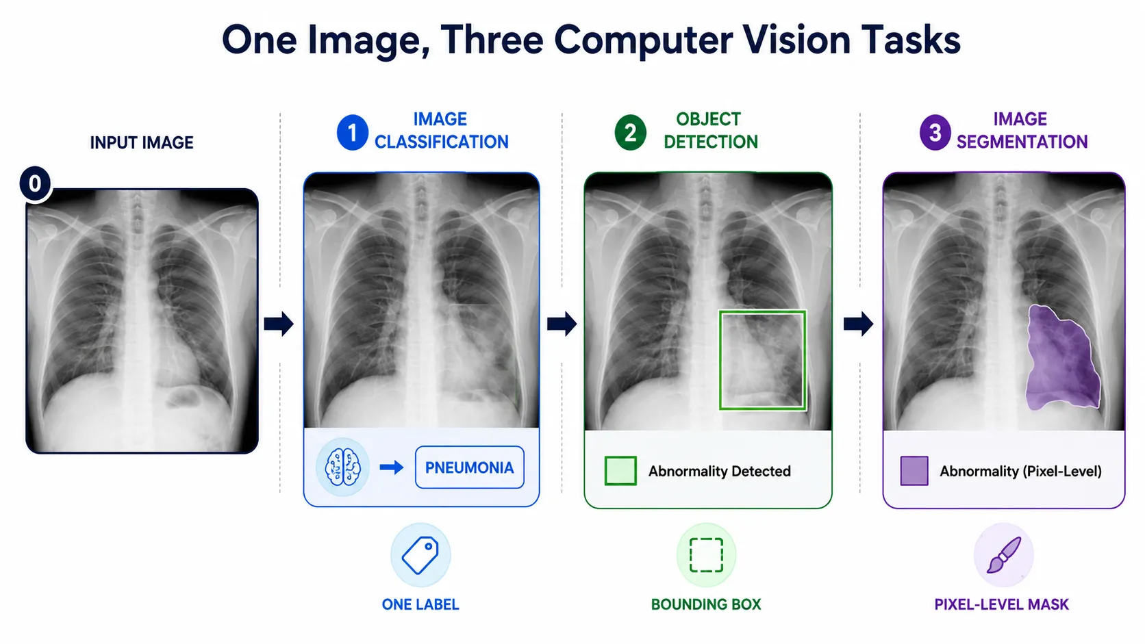
Image segmentation is a computer vision technique that divides an image into meaningful regions.
Instead of predicting one label for the entire image, a segmentation model tries to understand what individual pixels belong to.
Think about a photo containing a person, a car, a road, trees, and the sky.
A normal image classification model may recognize that the image contains a car.
An object detection model can go one step further and draw a box around that car.
Image segmentation goes even deeper. It can identify the exact pixels that belong to the car.
In simple words:
Classification tells us what is in an image.
Object detection tells us what it is and roughly where it is.
Image segmentation tells us exactly which pixels belong to it.
This difference becomes especially important in healthcare.
A rectangle around a brain tumor may include healthy tissue along with the tumor. For medical analysis, doctors often need the actual shape and boundaries of the abnormal region.
A segmentation model can produce a segmentation mask, where pixels predicted as tumor are marked separately from pixels belonging to normal brain tissue.
What Is U-Net?
U-Net is a deep learning architecture designed for image segmentation, especially biomedical image segmentation.
It was introduced by Olaf Ronneberger, Philipp Fischer, and Thomas Brox in 2015. The original architecture was developed for biomedical images and used a contracting path to understand image context and an expanding path to recover precise location information.
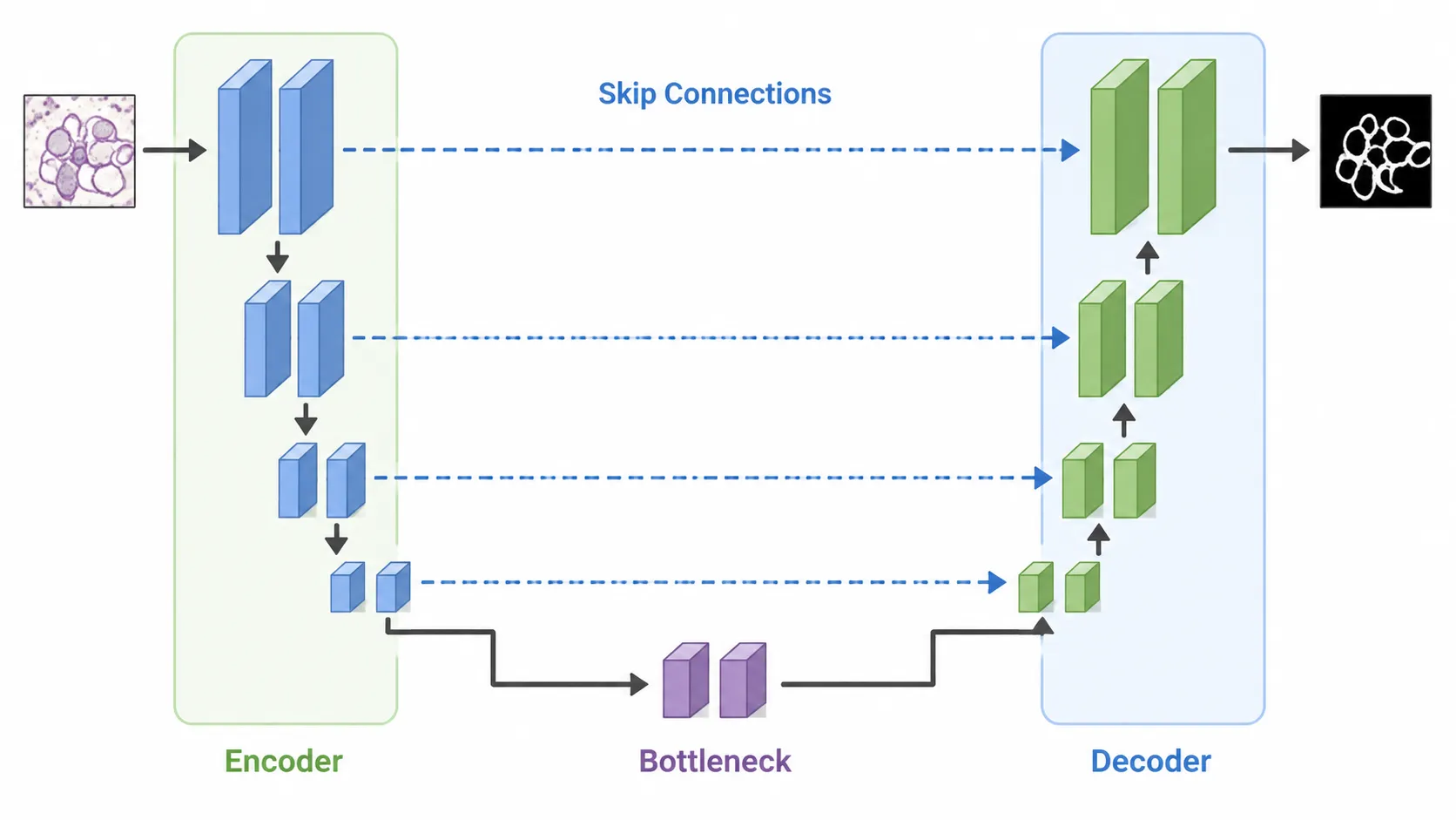
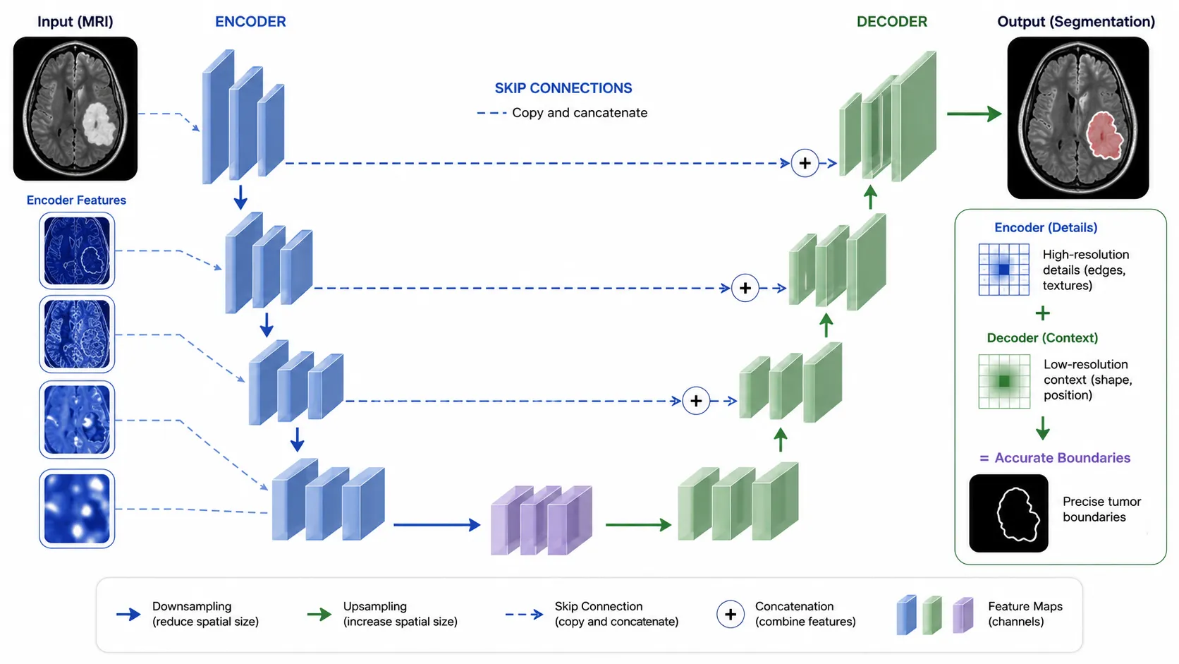
The name “U-Net” comes from the shape of its architecture.
If you draw the network layer by layer, the left side gradually becomes smaller, the network reaches a narrow middle section, and then the right side becomes larger again.
Together, these sections look similar to the letter U.
But the shape is not what makes U-Net powerful.
The important idea is that U-Net learns both:
what it is looking at and where that object is located.
This combination makes it particularly suitable for tasks where accurate boundaries matter.
Why Was U-Net Needed?
Traditional convolutional neural networks are excellent at learning visual patterns.
For example, deeper layers of a CNN may learn that a particular combination of shapes and textures looks like a tumor.
However, there is a problem.
As information travels deeper into a normal CNN, the feature maps usually become smaller. This helps the model understand high-level patterns, but some exact location information can disappear.
For classification, that may not be a major problem.
If the task is simply:
“Does this MRI contain a tumor?”
the model does not need to know the exact boundary.
But segmentation asks a much harder question:
“Which exact pixels belong to the tumor?”
U-Net was designed to preserve and recover this spatial information.
Real-World Example: Segmenting a Brain Tumor From an MRI Scan
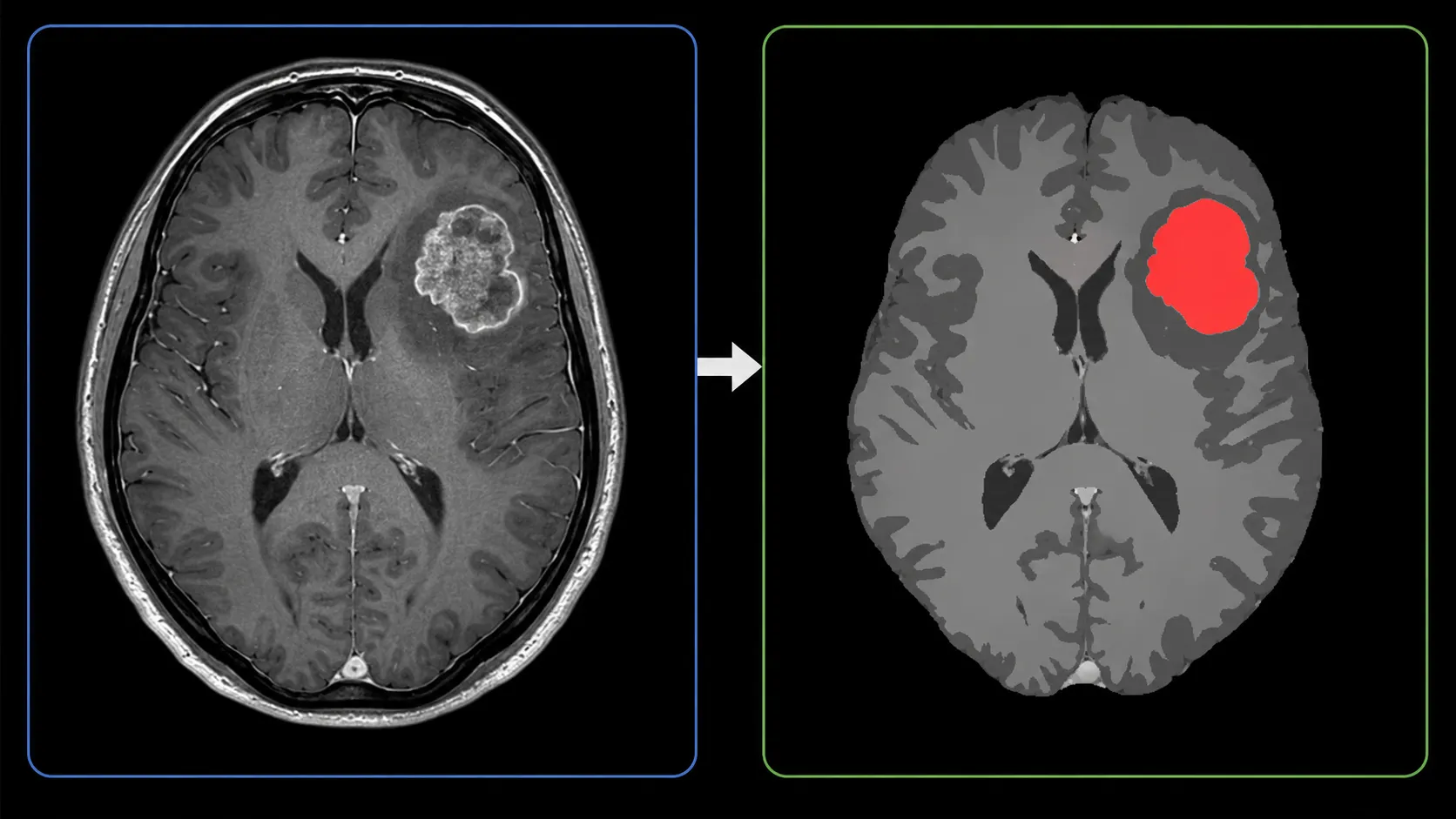
Suppose a hospital has an MRI scan of a patient's brain.
Inside the scan is a tumor that does not have a perfect circular or rectangular shape. Its boundary may be uneven, and some parts may look similar to surrounding tissue.
A radiologist can manually outline the tumor, but manual segmentation requires expertise and can take considerable time.
An automated brain tumor segmentation using U-Net system approaches the problem differently.
First, the MRI image is given to the network.
The model begins extracting visual features.
Early layers may notice simple information such as edges, intensity differences, and small patterns.
Deeper layers combine those simple features into more meaningful information.
The model gradually learns patterns that can help distinguish abnormal tissue from other structures in the brain.
After understanding those features, U-Net reconstructs the spatial information and produces an output mask.
The final result may look like the original MRI with the suspected tumor region highlighted.
This is why medical image segmentation using deep learning is different from simple image recognition. The goal is not only to recognize a disease-related pattern but also to locate its boundaries.
Recent research continues to use U-Net and its variants for MRI brain tumor segmentation. Reviews covering studies from recent years describe U-Net-based architectures as an important family of models for tumor segmentation and discuss their use with benchmark datasets such as BraTS.
How Does the U-Net Architecture Work?
U-Net can be understood through three important ideas:
The encoder understands the image.
The decoder rebuilds the location information.
Skip connections connect information from both sides.
Let us start with the encoder.
The Encoder: Learning What Is Inside the Image
The left side of U-Net is called the encoder, sometimes known as the contracting path.
Its job is to examine the input image and learn useful features.
Imagine giving the network a brain MRI.
At the beginning, the model sees raw pixel values.
After passing through convolution layers, it starts learning patterns such as edges and small shapes.
As the information moves deeper into the encoder, the network can learn more complex patterns.
At the same time, the width and height of the feature maps are gradually reduced.
You can think of this process like zooming out from a detailed map.
Some fine details become smaller, but the model gains a better understanding of the bigger picture.
For a brain MRI, this deeper information can help the network understand the relationship between different tissues and suspicious regions.
But reducing the image creates another challenge.
The network must eventually return from this compressed representation to a full-sized segmentation mask without losing the exact location of important features.
That is where the other half of U-Net becomes essential.
The Decoder: Turning Features Back Into a Segmentation Map
After the encoder understands the important features inside the MRI scan, U-Net needs to answer another question:
Where exactly are those features located?
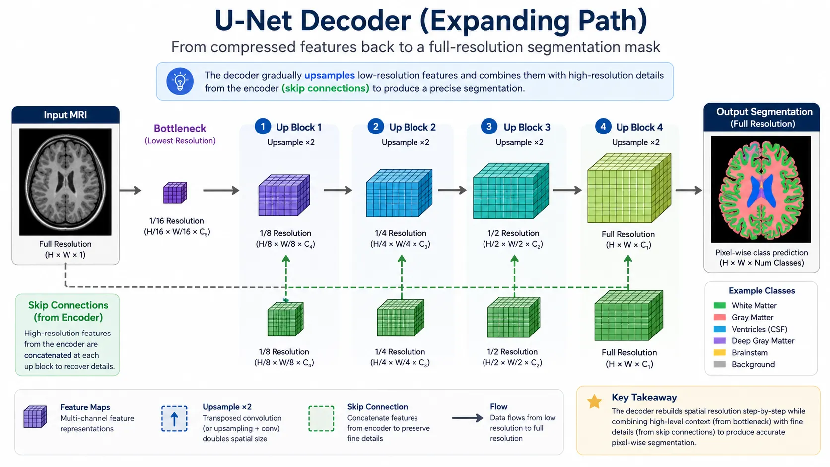
This job belongs to the decoder, also called the expanding path.
Remember what happened inside the encoder. The image became smaller as it moved deeper into the network. That helped the model understand larger patterns, but some fine location details became harder to preserve.
The decoder reverses this process.
Instead of reducing the feature maps, it gradually increases their size. This process is called upsampling.
Imagine looking at a small map of a city and then slowly zooming in until individual streets become visible again.
The decoder follows a similar idea.
It takes the learned features from the deeper part of the network and gradually brings them back toward the original image resolution.
For brain tumor segmentation, this is extremely important.
The model may already understand that a certain area looks like abnormal tissue, but now it must rebuild enough spatial detail to identify the shape and boundary of that area.
Skip Connections: The Feature That Makes U-Net Special
Here comes one of the most important ideas in the U-Net architecture: skip connections.
Instead of forcing the decoder to rebuild everything from compressed information alone, U-Net directly sends information from the encoder to matching layers in the decoder.
Think of it like this.
Suppose you are solving a puzzle. You first study the complete picture, then someone gives you smaller clues about the exact edges and shapes.
You would probably solve the puzzle more accurately because you have both:
the bigger picture and the small details.
Skip connections provide something similar to U-Net.
The deeper layers help the network understand what it is seeing.
Earlier encoder layers contain more information about where edges, shapes, and small details appeared.
U-Net combines these two types of information.
That is why skip connections can help the decoder produce more detailed segmentation boundaries.
For an MRI scan, this can be valuable when the tumor has an irregular border rather than a clean circular shape.
U-Net Architecture Step by Step
Now let us put everything together.
Imagine that an MRI scan enters a trained U-Net model.
Step 1: The MRI Image Enters the Network
The process starts with the input image.
Depending on the system, this may be one MRI slice or information prepared from multiple MRI sequences.
At this point, the network does not see a “brain” or a “tumor” in the way a human does.
It receives numerical pixel values.
Step 2: Convolution Layers Find Visual Features
The encoder passes the image through convolution operations.
At early stages, the network can learn simple patterns such as edges, intensity changes, textures, and shapes.
Deeper layers combine these smaller patterns into more useful representations.
For example, instead of simply noticing a bright region, the network may learn whether that region appears in a context that is commonly associated with a particular tumor area.
Step 3: Downsampling Builds Context
As information moves deeper into the encoder, the spatial size becomes smaller.
This helps the network look beyond individual pixels and understand a wider area of the image.
You can think of this as moving from:
“Something unusual is happening in these pixels”
to:
“This unusual region appears in this part of the brain and has these surrounding patterns.”
Step 4: The Bottleneck Holds Deep Features
At the bottom of the U-shaped network is the bottleneck.
This is the bridge between the encoder and decoder.
By this stage, the model has processed the image through several levels of feature extraction.
The representation is smaller than the original image, but it contains rich information learned from the input.
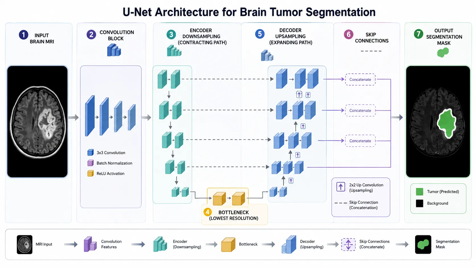
Step 5: The Decoder Upsamples the Features
Now the model begins moving through the expanding path.
The decoder increases the spatial resolution step by step.
Its goal is to transform the learned features into a detailed prediction that matches the location of structures in the original image.
Step 6: Skip Connections Bring Back Fine Details
At different decoder levels, information from the matching encoder levels is added.
This is the part beginners should remember.
The decoder is not working alone.
It receives deeper information about the meaning of the image while also receiving finer features from earlier encoder stages.
Together, these features help U-Net decide more precisely where a target region begins and ends.
Step 7: U-Net Creates the Segmentation Mask
At the end of the network, U-Net produces a prediction for the image pixels.
For a simple tumor-versus-background task, each pixel may be assigned a probability representing how likely it is to belong to the tumor.
Those predictions can then be converted into a segmentation mask.
A simple mask might contain:
background pixels representing normal or non-target areas,
and foreground pixels representing the predicted tumor region.
The important point is that the model is not simply saying:
“Tumor present.”
It is trying to say:
“These specific pixels are likely to belong to the tumor.”
What Does the Final Brain Tumor Segmentation Look Like?
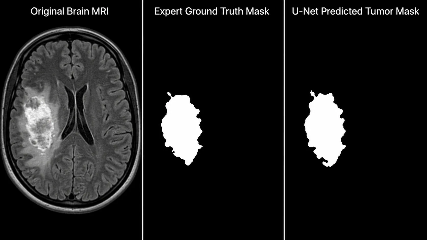
Imagine placing three images side by side.
The first is the original brain MRI.
The second is a manually created tumor mask prepared by an expert.
The third is the mask predicted by the U-Net model.
If the model performs well, the predicted region should closely follow the reference tumor area.
This allows researchers to measure how closely the prediction overlaps with the expected segmentation.
One commonly used evaluation measure in brain tumor segmentation is the Dice score.
You do not need to worry about the mathematical formula yet.
For now, think of Dice score as a way of asking:
“How much does the predicted tumor region overlap with the correct tumor region?”
A stronger overlap generally means a better segmentation result.
The BraTS brain tumor benchmark, for example, has widely used Dice-based evaluation along with other measures to compare segmentation methods.
However, a high score alone does not automatically mean that an AI system is ready to make clinical decisions.
Real MRI data can vary between hospitals, scanners, imaging protocols, tumor types, and patient populations.
That means a model that performs well on a research dataset still needs careful validation before clinical use.
And this leads to the next important question:
Why has U-Net become such a popular starting point for medical image segmentation, and what makes it different from ordinary CNN architectures?
Why Is U-Net So Popular for Medical Image Segmentation?
U-Net became popular because medical images create a difficult problem.
In normal computer vision projects, developers may have thousands or even millions of labeled images. Medical datasets are different.
Creating a correct segmentation mask often requires a trained doctor or medical expert to manually mark the important region. Because this takes time and specialist knowledge, high-quality labeled medical images can be limited.
The original U-Net was designed with this problem in mind. Its training strategy used data augmentation to make better use of available annotated images.
Another major advantage is its ability to combine high-level understanding with precise location information.
The encoder learns what important patterns look like.
The decoder restores spatial resolution.
Skip connections bring useful details from earlier layers directly into the decoding process.
This combination gives U-Net a strong foundation for tasks where the exact shape of an object matters.
U-Net vs a Normal CNN
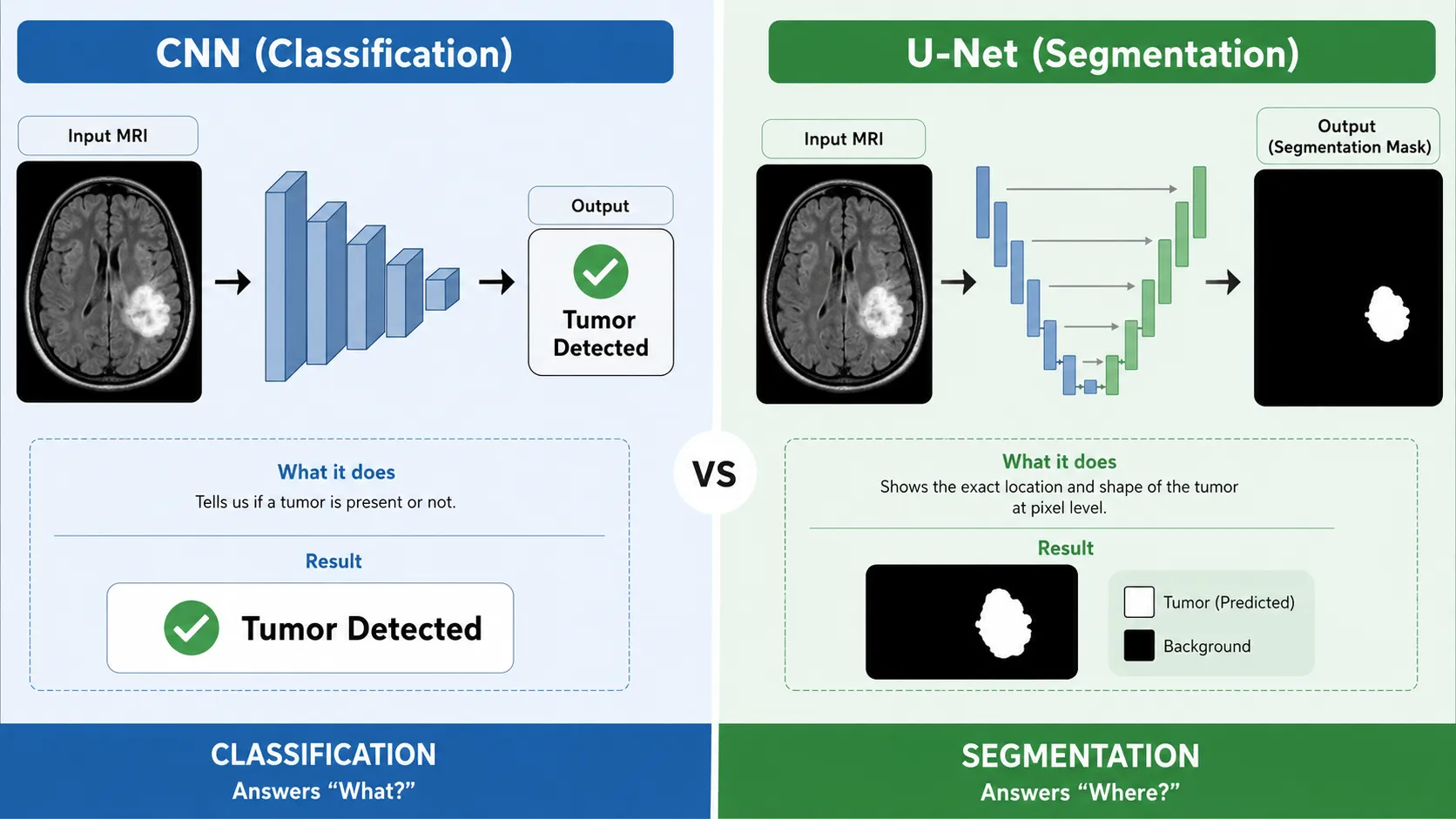
A normal convolutional neural network (CNN) and U-Net can both learn visual patterns, but they usually solve different problems.
Imagine showing an MRI scan to a classification CNN.
Its final answer might be:
“Brain tumor detected.”
That can be useful, but it does not tell us the exact location or shape of the tumor.
Now give the same MRI to a trained U-Net segmentation model.
Instead of returning only one label, the model can create a pixel-level mask showing the predicted tumor region.
So the main difference is simple:
A classification CNN answers:
“What is inside this image?”
U-Net segmentation answers:
“What is inside this image, and exactly which pixels belong to it?”
This is why U-Net for brain tumor segmentation is more suitable when boundaries, shape, and location matter.
How Is a U-Net Model Trained?
Before U-Net can segment a new MRI scan, it must learn from examples.
Suppose we have a collection of brain MRI scans.
For every training scan, experts provide a corresponding ground-truth segmentation mask showing the actual tumor region.
The model receives the MRI scan and produces its own predicted mask.
At first, that prediction may be poor.
The training system compares the predicted mask with the correct mask and calculates how different they are.
This difference is represented through a loss function.
The model then updates its internal weights.
It repeats this process across many training examples.
Over time, the network learns which image patterns are useful for separating tumor tissue from other regions.
Why the Loss Function Matters
One challenge in brain tumor segmentation is that the tumor may occupy only a small part of the complete MRI image.
Imagine an MRI containing 100,000 pixels while only a small percentage belong to the tumor.
A model could classify most pixels as background and still appear successful if we looked only at basic accuracy.
That would be misleading.
For segmentation, we need methods that pay attention to the target region.
This is one reason Dice-based loss functions are commonly used in medical image segmentation research.
Dice focuses on the overlap between the predicted area and the actual target area.
Researchers also use approaches such as cross-entropy, weighted cross-entropy, generalized Dice loss, or combinations of different losses depending on the segmentation problem. Recent U-Net-based brain tumor studies continue to investigate these loss functions because class imbalance remains an important challenge.
How Do We Know If the Segmentation Is Good?
Training a model is not enough.
We also need to evaluate its predictions.
Dice Score
The Dice score measures how strongly the predicted segmentation overlaps with the correct segmentation.
A Dice score closer to 1 means stronger overlap.
For example, imagine that a radiologist marks the actual tumor region and U-Net predicts almost the same region.
The Dice score would be high.
If the predicted mask misses large sections of the tumor or includes many incorrect areas, the score would fall.
Hausdorff Distance
Another useful measurement is the Hausdorff distance, especially when researchers want to study differences between segmentation boundaries.
In brain tumor segmentation benchmarks such as BraTS, Dice and Hausdorff-based measurements are commonly used alongside metrics such as sensitivity and specificity.
This matters because one number cannot always describe the complete quality of a medical segmentation.
A model might achieve good overall overlap while still making mistakes around an important boundary.
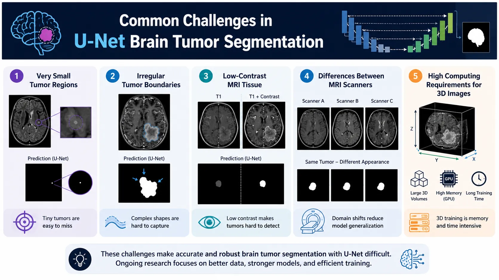
Limitations of U-Net for Brain Tumor Segmentation
U-Net is powerful, but it is not perfect.
Understanding its limitations is just as important as understanding its strengths.
Small and Irregular Tumor Regions Can Be Difficult
Brain tumors do not always have simple shapes.
Some regions may be extremely small, irregular, or visually similar to nearby tissues.
These difficult areas can still cause segmentation errors.
MRI Scans Can Differ Between Hospitals
An MRI scan produced by one hospital may not look exactly like an MRI from another hospital.
Different scanners, settings, imaging protocols, and patient populations can change the appearance of the data.
A model trained on one dataset may therefore perform differently when it receives images from a new clinical environment.
This problem is often called domain shift or a generalization problem.
Recent research continues to identify cross-site generalization and irregular tumor subregions as important challenges for U-Net-based brain tumor segmentation.
Training Can Require Significant Computing Power
Basic 2D U-Net models can be relatively manageable, but medical imaging systems can become much heavier when working with complete 3D MRI volumes.
Larger images, deeper networks, 3D convolutions, and advanced U-Net variants can require substantial GPU memory and training time.
Popular U-Net Variants
The success of the original architecture has inspired many modified versions.
For example, 3D U-Net can process volumetric information rather than treating every MRI slice completely independently.
Attention U-Net introduces attention mechanisms that can help the network focus on relevant regions.
U-Net++ uses redesigned nested skip pathways to improve feature fusion between encoder and decoder stages.
Researchers have also combined U-Net-style architectures with residual connections, transformers, deep supervision, and other techniques.
However, a newer architecture is not automatically better for every dataset.
The best choice depends on the available data, computing resources, image type, required accuracy, and real-world use case. Reviews of U-Net-based brain MRI segmentation continue to find multiple successful variants rather than one architecture that solves every situation.
From MRI Scan to Tumor Mask: The Complete Picture
Let us return to the patient MRI example from the beginning.
The MRI enters the trained U-Net.
The encoder studies the image and learns important features.
The bottleneck captures deeper context.
The decoder begins rebuilding spatial resolution.
Skip connections restore useful information from earlier layers.
Finally, the network predicts which pixels are likely to belong to the tumor.
Those predictions form the segmentation mask.
That mask can then be compared with expert annotations, measured using segmentation metrics, or used as one component of a larger medical imaging workflow.
The important idea is simple:
U-Net does not only try to recognize what it sees. It tries to understand where it is, pixel by pixel.
Final Thoughts
U-Net changed image segmentation by combining a simple idea with a very practical architecture.
Its encoder learns the meaning of visual patterns.
Its decoder restores their location.
Its skip connections help preserve details that could otherwise disappear.
That is why learning U-Net image segmentation is useful far beyond one brain MRI example.
The same basic idea has influenced segmentation systems for organs, cells, lesions, tumors, satellite images, industrial defects, and many other computer vision problems.
If you are beginning your journey into deep learning image segmentation, do not start by memorizing every convolution, filter size, or mathematical equation.
Remember the main story first:
Encoder understands.
Decoder reconstructs.
Skip connections recover details.
The final mask identifies the target pixel by pixel.
Once this picture is clear, understanding advanced U-Net architectures becomes much easier.
Frequently Asked Questions About U-Net Image Segmentation
What Is U-Net in Image Segmentation?
U-Net is a deep learning architecture designed for pixel-level image segmentation. It uses an encoder to learn important features, a decoder to rebuild the image resolution, and skip connections to transfer useful details between both sides of the network.
Instead of only recognizing what is inside an image, U-Net can identify exactly which pixels belong to a particular object or region.
How Does U-Net Work for Image Segmentation?
U-Net first sends the input image through an encoder.
The encoder gradually extracts important visual features while reducing the size of the feature maps.
The decoder then increases the resolution again and combines its features with information received from earlier encoder layers through skip connections.
Finally, the network creates a segmentation mask that identifies the target region pixel by pixel.
Why Is U-Net Used for Medical Image Segmentation?
U-Net is widely used in medical image segmentation because medical tasks often require accurate boundaries rather than only image-level predictions.
For example, detecting that a brain MRI contains a tumor is useful, but doctors and researchers may also need to know the tumor's exact shape, size, and location.
U-Net is designed to preserve spatial details while also learning deeper visual patterns, making it suitable for tasks involving tumors, organs, lesions, cells, and other medical structures.
How Does U-Net Segment Brain Tumors From MRI Scans?
A trained U-Net receives an MRI scan and analyzes its visual patterns.
The encoder learns features that may help distinguish tumor tissue from surrounding areas. The decoder then restores the spatial information and produces a pixel-level prediction.
The result is a segmentation mask showing the region that the model predicts belongs to the brain tumor.
This mask can then be compared with an expert-created reference mask to evaluate how accurately the model has identified the tumor.
What Are Skip Connections in U-Net?
Skip connections directly connect encoder layers with matching decoder layers.
They allow the decoder to reuse detailed information that may otherwise be lost during downsampling.
A simple way to understand this is:
The deeper layers tell the model what it is looking at, while earlier layers help tell it where the details are located.
Combining both helps U-Net produce more precise segmentation boundaries.
What Is a Segmentation Mask?
A segmentation mask is an image-like output that identifies which pixels belong to a target object or region.
For brain tumor segmentation, the mask can highlight pixels predicted as tumor while treating the remaining pixels as background or other tissue.
Depending on the task, a segmentation mask can contain two classes or several different classes.
What Is the Difference Between U-Net and a Normal CNN?
A normal classification CNN usually produces one prediction for an entire image.
For example:
CNN: “This MRI contains a brain tumor.”
U-Net produces a pixel-level result.
For example:
U-Net: “These pixels represent the predicted tumor region.”
That makes U-Net more suitable when the exact location and shape of an object are important.
What Is the Dice Score in Image Segmentation?
The Dice score measures the overlap between a predicted segmentation and the correct reference segmentation.
If the predicted tumor mask closely matches the expert-created tumor mask, the Dice score will be higher.
A value closer to 1 generally represents stronger overlap.
Because medical images may contain a very small target region compared with the background, Dice-based measures are commonly used when evaluating segmentation models.
Is U-Net Only Used for Brain Tumor Segmentation?
No.
Brain tumor segmentation is only one example.
U-Net and U-Net-based architectures have been used for many tasks, including organ segmentation, cell segmentation, lesion detection, blood vessel segmentation, lung segmentation, satellite imagery, road segmentation, and industrial defect detection.
The basic U-Net idea can be applied whenever a model needs to identify precise regions inside an image.
Is U-Net Still Useful for Image Segmentation?
Yes.
Many newer segmentation architectures now exist, including U-Net++, Attention U-Net, nnU-Net, transformer-based networks, and foundation-model approaches.
However, U-Net remains an important architecture to learn because its encoder-decoder design and skip connections form the foundation of many later segmentation models.
For a beginner learning medical image segmentation, understanding U-Net makes many advanced architectures much easier to understand.


