


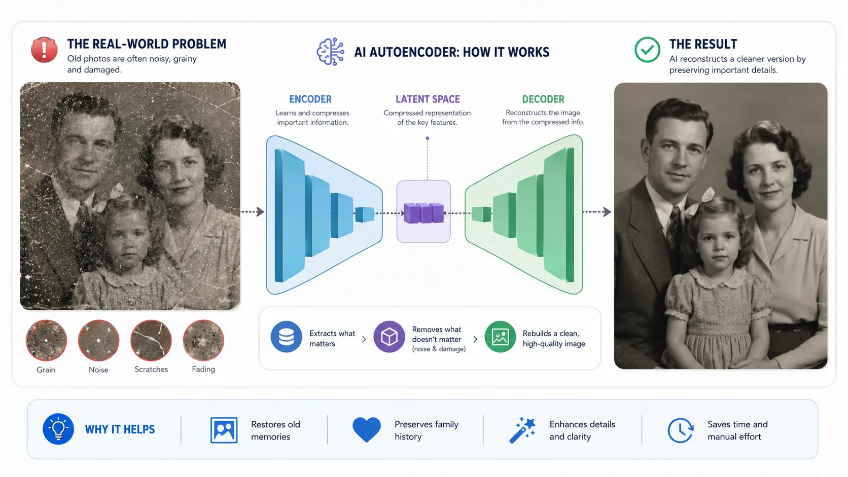
Imagine finding an old family photo that has been sitting in a drawer for years. The people in the picture are still visible, but the image has grain, tiny white spots, scratches, and random noise.
You know what the original scene should roughly look like. The problem is removing the unwanted details without destroying the faces, clothes, and background that actually matter.
This is surprisingly close to one of the problems an autoencoder in deep learning can learn to solve.
Autoencoders are neural networks that learn how data is structured. Instead of simply looking at an image and deciding whether it contains a cat, car, or person, an autoencoder tries to understand enough about the input to rebuild it.
That simple idea leads to some very useful applications.
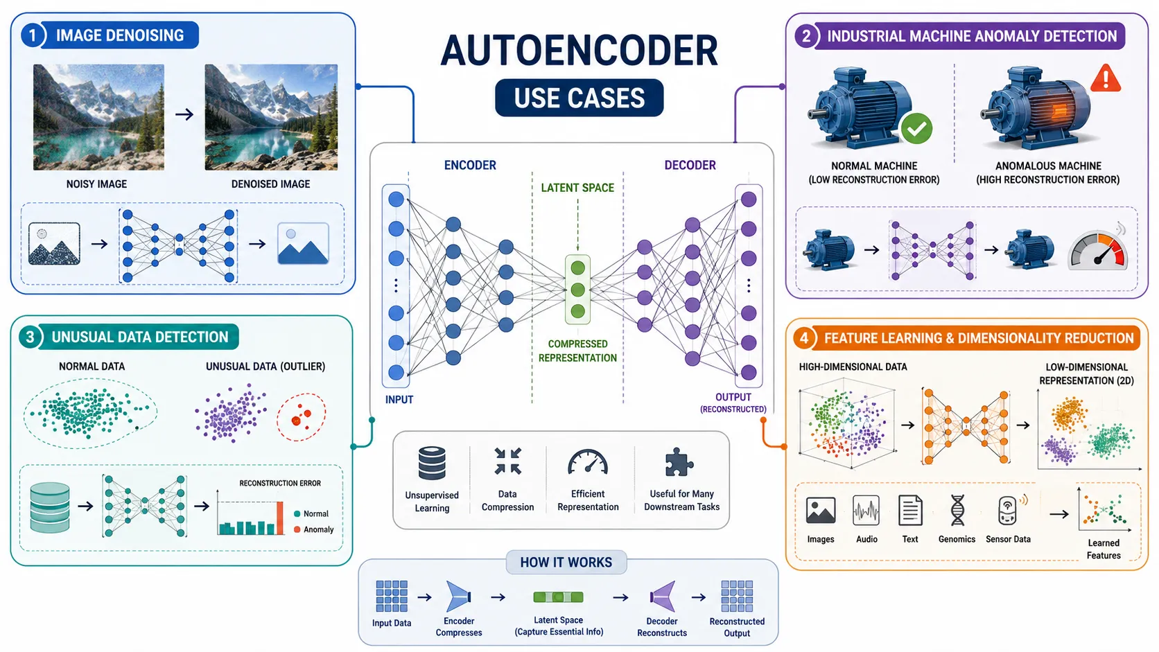
Autoencoders can help reduce noise in images, learn useful features, compress complex data into smaller representations, and even identify unusual patterns that may indicate fraud, equipment problems, or abnormal sensor readings.
And the interesting part is that the basic idea is much easier to understand than its name makes it sound.
What Is an Autoencoder?
An autoencoder is a type of neural network that receives some data, creates a smaller internal representation of it, and then tries to reconstruct the original data.
Think about sending a large suitcase through an airport baggage system.
Before the suitcase can fit into a smaller storage space, you may have to organize it carefully and keep only the information about where everything belongs. Later, when you open it again, you want to recover the important contents as accurately as possible.
An autoencoder works in a similar way.
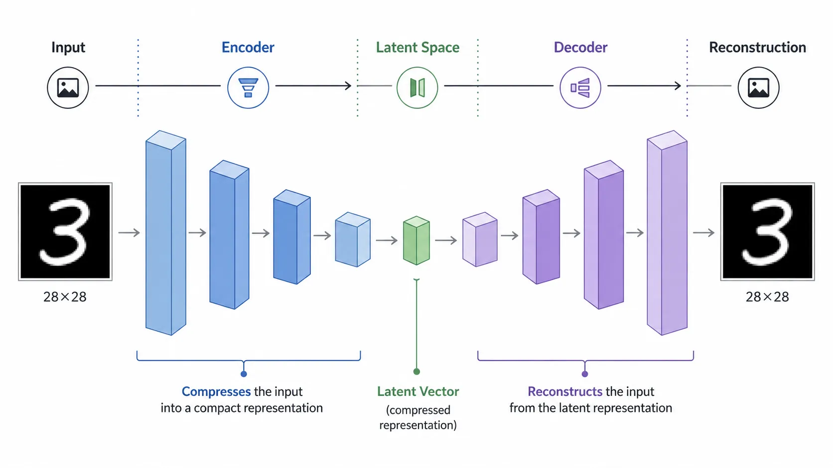
It takes an input such as an image and passes it through an encoder. The encoder converts that input into a compact representation.
That compact version then moves through a decoder, which attempts to rebuild the original input.
In simple form, the process looks like this:
Input → Encoder → Compressed Representation → Decoder → Reconstructed Output
The model then compares the reconstructed output with the original input.
If the reconstruction is poor, the model adjusts its internal weights and tries again. With repeated training, it becomes better at preserving the patterns that matter.
This difference between the original input and reconstructed output is called reconstruction error or reconstruction loss.
The Three Main Parts of an Autoencoder
To understand how autoencoders work, you mainly need to understand three parts: the encoder, the bottleneck, and the decoder.
Encoder
The encoder receives the original data and gradually converts it into a smaller representation.
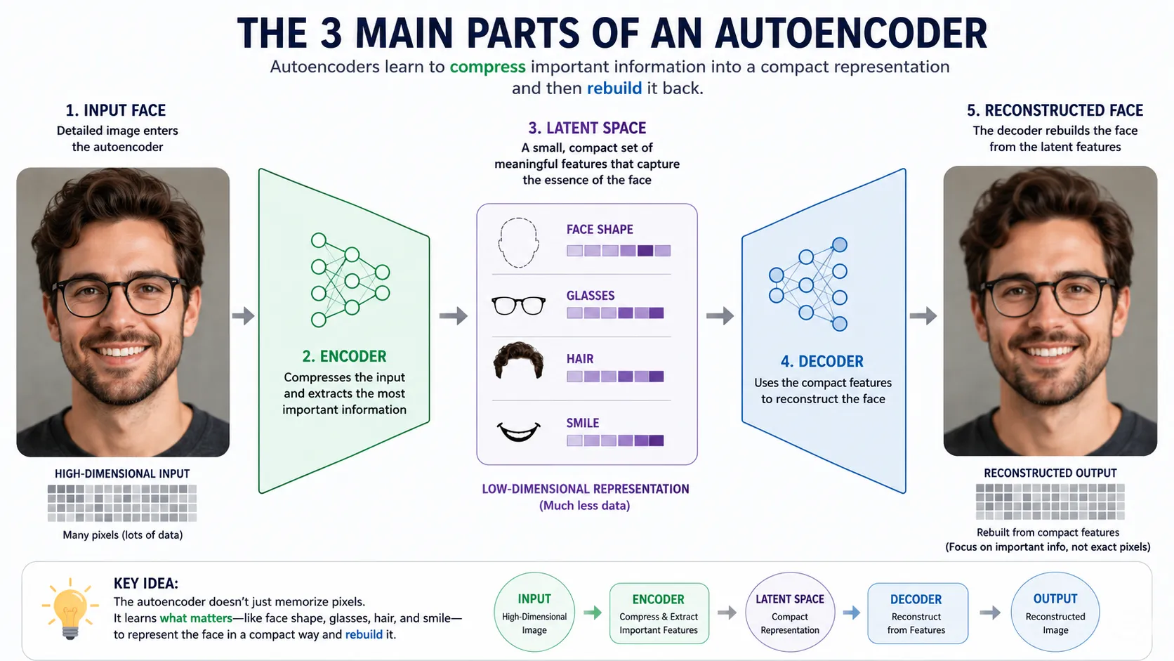
Suppose you give the network a photograph of a human face.
The raw image contains thousands or even millions of pixel values. But not every individual pixel is equally useful.
Patterns such as the shape of the eyes, edges of the face, hair structure, lighting, and general position of facial features carry much more useful information.
During training, the encoder learns how to represent important patterns using fewer values.
You can think of it as making detailed notes from a long chapter instead of memorizing every single sentence.
The goal is not simply to make the data smaller. The goal is to keep enough useful information to rebuild it later.
Bottleneck or Latent Space
After the encoder compresses the data, it reaches a small internal representation commonly called the bottleneck, encoding, or latent representation.
The term may sound technical, but the idea is straightforward.
Imagine describing a face without sending the photograph itself.
You might describe:
“Round face, dark hair, glasses, smiling.”
That short description obviously does not contain every pixel from the original photo, but it captures several important characteristics.
The latent space works somewhat like that compressed description.
It represents important patterns learned by the neural network without keeping every detail in its original form.
This is also one reason autoencoders can be useful for feature learning and dimensionality reduction.
Decoder
The decoder performs the opposite job.
It receives the compressed representation and attempts to recreate the original input.
If the encoder stored useful information, the decoder should be able to create an output that looks reasonably close to the original data.
During training, the model repeatedly asks one important question:
“How different is my reconstruction from the original?”
That difference becomes the learning signal.
A large reconstruction error means the network needs improvement. A smaller error means its internal representation is doing a better job of preserving useful information.
A Simple Real-Life Example: Compressing a Handwritten Number
Imagine showing an autoencoder thousands of handwritten numbers.
Every person writes the number 8 slightly differently.
Some write it wide. Some write it narrow. Some use thick strokes, while others write lightly.
An autoencoder does not need to memorize every individual pixel arrangement.
Instead, while learning to reconstruct the images, it begins to capture recurring patterns such as curves, edges, stroke positions, and shapes.
The encoder turns the image into a smaller representation.
The decoder then uses that representation to rebuild the handwritten digit.
If important details were lost during compression, the reconstructed image may look distorted. The reconstruction loss tells the network how far its result was from the original.
Training repeats this process many times until the network becomes better at representing the underlying structure of the data.
This concept is important because it explains why an autoencoder is more than a simple image copier.
Why Not Just Copy the Input?
At first, this creates an obvious question.
If the desired output is the same as the input, why build a neural network at all?
Because simply copying the data teaches us almost nothing.
A useful autoencoder is designed or trained in a way that prevents easy copying. One common approach is forcing information through a smaller bottleneck.
If a network receives 1,000 pieces of information but can pass only a much smaller representation through its middle layer, it has to decide what matters.
It cannot preserve everything equally.
That pressure encourages the model to learn useful structure.
And this becomes even more interesting when we deliberately damage the input before giving it to the model.
Instead of saying:
“Here is a clean photo. Copy it.”
we can say:
“Here is a noisy version of the photo. Reconstruct the clean original.”
That small change gives us a denoising autoencoder.
And this is where our old-photo example starts becoming a real deep-learning solution.
What Is a Denoising Autoencoder?
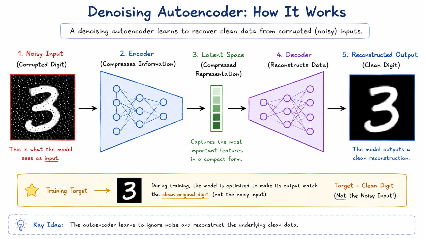
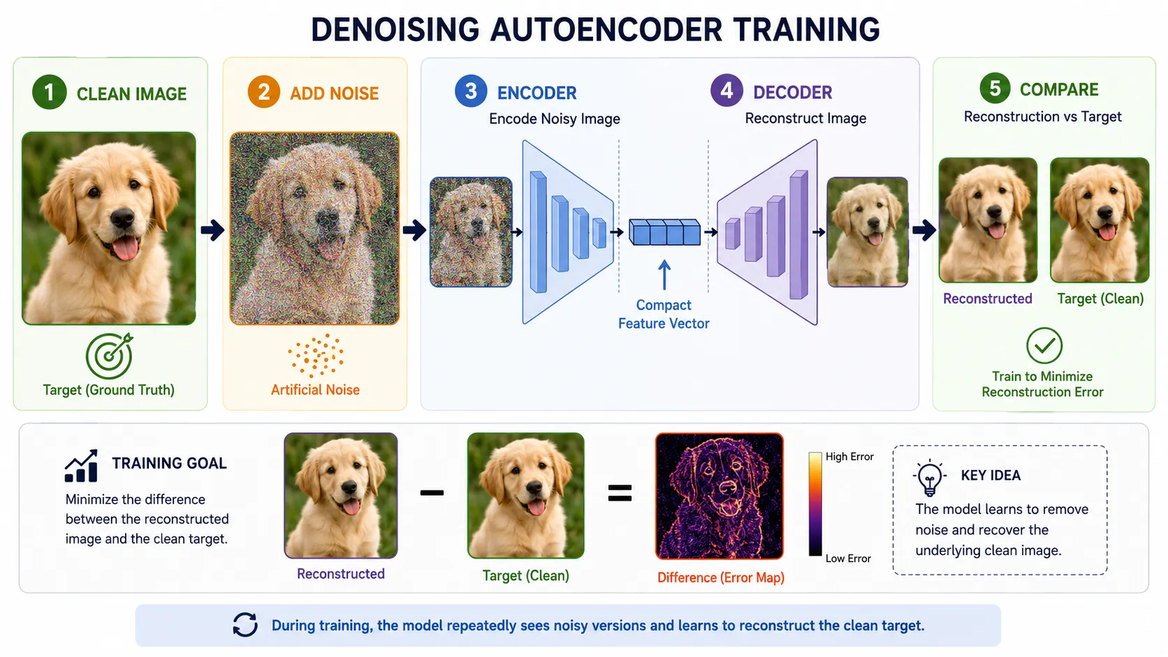
A denoising autoencoder is an autoencoder trained to recover clean data from a damaged or noisy version of that data.
Instead of giving the network a clean image and asking it to reproduce the same clean image, we deliberately add noise to the input.
The training process becomes:
Noisy Input → Encoder → Latent Representation → Decoder → Clean Output
The target is still the original clean image.
This small difference completely changes what the model learns.
A normal autoencoder may become good at reproducing whatever it receives. A denoising autoencoder has a harder job. It must learn which patterns belong to the real image and which patterns are just unwanted noise.
Imagine someone sends you this sentence:
“I l*ve mach!ne learn#ng.”
Even with the strange symbols, you can probably understand that the intended sentence is:
“I love machine learning.”
You can do that because you understand the structure of language.
A denoising autoencoder tries to develop a similar understanding of patterns in its training data.
How Does a Denoising Autoencoder Work?
Let us return to our old photograph.
Suppose you have thousands of clean photographs available for training.
You create slightly damaged versions of those images by adding random noise. The noisy images become the inputs, while the original clean images remain the expected outputs.
The model now repeatedly sees examples such as:
Noisy face → Clean face
Noisy building → Clean building
Noisy handwritten digit → Clean handwritten digit
Every time the network produces an output, it compares its reconstruction with the clean target.
If the result is poor, the network adjusts itself.
After seeing enough examples, it starts learning which visual structures are common and which random changes should usually be ignored.
Let us break this process down.
Step 1: Start With Clean Training Data
First, we need examples representing the type of data we want the model to understand.
For an image denoising project, these could be photographs, handwritten digits, medical images, product images, or another visual dataset.
Suppose we are training the model using handwritten digits.
The dataset contains thousands of clean images of numbers from 0 to 9.
Step 2: Add Noise to the Images
Next, artificial noise is added to the clean images.
A clean handwritten 5, for example, may now contain random light and dark pixels around its shape.
This noisy version becomes the input.
The original image remains the target.
So the model is not being asked to reproduce the noise.
It is being asked to remove it.
One commonly used form is Gaussian noise, where random changes are added to pixel values. The exact mathematics is less important for a beginner than the main idea: we intentionally disturb the image so the network learns how to recover useful information.
Step 3: The Encoder Reads the Noisy Image
The noisy image enters the encoder.
The encoder gradually reduces the information into a smaller representation.
But now it faces an interesting challenge.
Some information comes from the actual object, while some comes from random noise.
Because random noise does not follow the same stable patterns as the real training data, the network can gradually learn representations that focus more on meaningful structures.
For a handwritten number, those structures may include curves, lines, edges, and the overall shape of the digit.
Step 4: The Decoder Rebuilds the Clean Image
The decoder receives the encoded representation and tries to reconstruct the clean target.
If the input contained noise around a handwritten number, the desired output should contain the digit while reducing that unwanted noise.
During early training, the result may look poor.
But each mistake gives the network useful feedback.
Reconstruction Loss: How the Model Knows It Made a Mistake
A neural network needs a way to measure how good or bad its output is.
For autoencoders, this is handled through reconstruction loss.
Suppose the original clean image is A.
The denoising autoencoder receives a noisy version of A and produces reconstructed image B.
The training process measures the difference between A and B.
If B is very different from A, reconstruction loss is high.
If B is very similar to A, reconstruction loss is lower.
The goal during training is to reduce this reconstruction error.
Different projects may use different loss functions depending on the type of data and model. For images, techniques such as mean squared error or binary cross-entropy can be used in suitable setups.
For now, remember one simple idea:
The model improves by learning from the difference between what it produced and what the clean output should have been.
That idea will become extremely important again when we use autoencoders for anomaly detection.
Old Photo Noise Removal: A Real-World Scenario
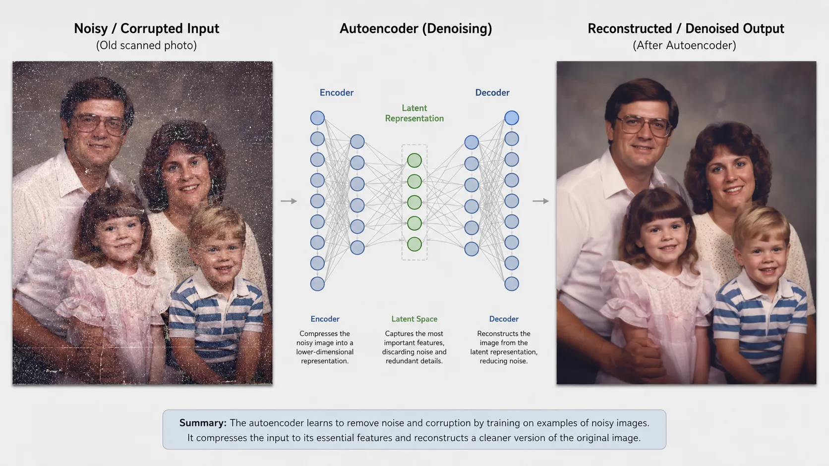
Imagine a photo-restoration company receives thousands of scanned family photographs.
Many photographs contain grain, faded regions, scanning noise, or tiny unwanted marks.
Cleaning every photograph manually could take a lot of time.
A deep-learning system could be trained using examples of clean and noisy images.
During training, the denoising autoencoder learns to map damaged-looking inputs toward cleaner versions.
When a new noisy image arrives, the process may look like this:
Old noisy photo → Denoising autoencoder → Cleaner reconstructed photo
The system does not simply apply the same correction to every pixel.
Its usefulness comes from learning patterns from training data.
If the model has learned what meaningful visual structures generally look like, it can attempt to preserve those structures while reducing unwanted random patterns.
This same basic idea can be useful in other areas too.
Medical scans may contain noise.
Camera images taken in difficult conditions can contain unwanted visual disturbance.
Scanned documents may contain random marks.
Sensor signals can also contain noisy measurements.
The data may change, but the core learning idea remains similar.
Autoencoder vs Denoising Autoencoder
The easiest way to remember the difference is to look at what enters the model.
A standard autoencoder usually learns:
Clean Input → Reconstruct Clean Input
A denoising autoencoder learns:
Corrupted Input → Reconstruct Clean Input
That means the denoising version is deliberately trained with damaged input.
Why?
Because we do not want the network to simply memorize how to copy pixels.
We want it to learn useful structure well enough to recover information even when the input is imperfect.
This makes denoising autoencoders an important example of representation learning.
The model is not explicitly told:
“This group of pixels represents an important edge.”
“This random dot is noise.”
“This curve belongs to the actual object.”
Instead, it learns useful patterns through the reconstruction task.
And once you understand this idea, another powerful use of autoencoders becomes much easier to understand.
Suppose we train an autoencoder almost entirely on normal data.
It becomes very good at reconstructing patterns similar to what it has already learned.
But what happens when we suddenly give it something very unusual?
Its reconstruction may become worse.
That difference gives us a clue that the input could be abnormal.
And that is the foundation of autoencoder anomaly detection.
How Autoencoders Detect Anomalies
An autoencoder can do more than clean noisy images.
It can also help us find unusual data.
This technique is called autoencoder anomaly detection.
The basic idea is simple.
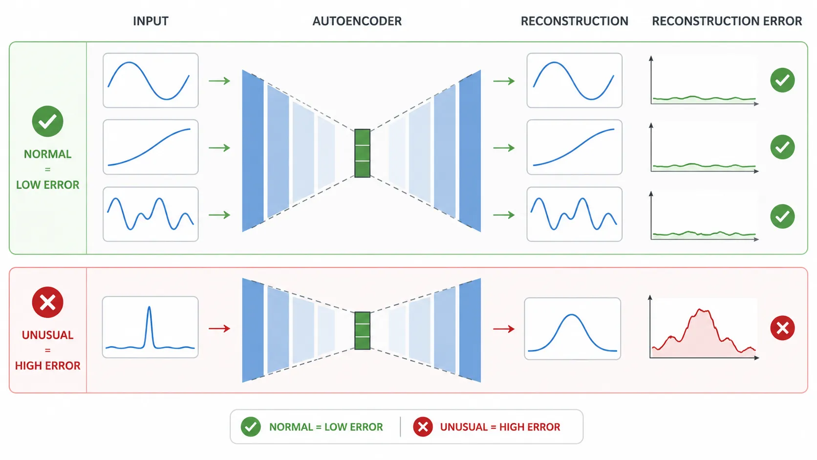
If an autoencoder is trained mostly on normal examples, it becomes good at reconstructing data that looks similar to those examples.
But when something very different appears, the model may struggle to rebuild it correctly.
That usually creates a larger reconstruction error.
And that error can become a warning signal.
Think about a worker who checks the same type of machine every day.
After months of experience, normal machine sounds become familiar.
If one morning the machine suddenly starts making a strange clicking sound, the worker may immediately notice that something feels different.
The worker may not know the exact fault yet, but the unusual pattern is enough to trigger attention.
An autoencoder can work in a similar way.
How Autoencoder Anomaly Detection Works
Suppose a factory has sensors installed on hundreds of machines.
Every few seconds, those sensors collect information such as:
temperature
vibration
pressure
motor speed
energy use
Most of the machines are working normally.
We train an autoencoder mainly using this normal sensor data.
During training, the network learns how normal machine behavior usually looks.
When normal data enters the model, it can often reconstruct it with a relatively small reconstruction error.
Now imagine that one machine develops a bearing problem.
Its vibration pattern changes.
The sensor data no longer looks like the normal patterns the model learned during training.
The autoencoder may fail to reconstruct that unusual input accurately.
As a result, the reconstruction error increases.
The system can then flag that reading for further investigation.
This does not automatically mean:
“The bearing is definitely broken.”
Instead, it means:
“This pattern looks unusual compared with what the model considers normal.”
That distinction is important.
Autoencoders can help identify suspicious cases, but a real production system may still need additional checks before making a final decision.
Reconstruction Error as an Anomaly Signal
Let us make the idea even simpler.
Imagine a model reconstructs a normal input almost perfectly.
The original data and reconstructed data are very close.
That means the reconstruction error is low.
Now another input enters the system.
This one contains an unusual pattern that the model has rarely or never seen before.
The reconstructed version is noticeably different from the original.
The reconstruction error becomes higher.
A system can use a reconstruction error threshold to decide when something should be treated as unusual.
For example:
If reconstruction error is below the chosen threshold, the input may be treated as normal.
If reconstruction error goes above the threshold, the input may be marked as a possible anomaly.
Choosing that threshold is an important part of building a reliable anomaly detection system.
If the threshold is too low, the system may produce too many false alarms.
If it is too high, important anomalies could be missed.
So the threshold should normally be selected by testing the model on suitable validation data.
Real-World Example: Detecting Unusual Transactions
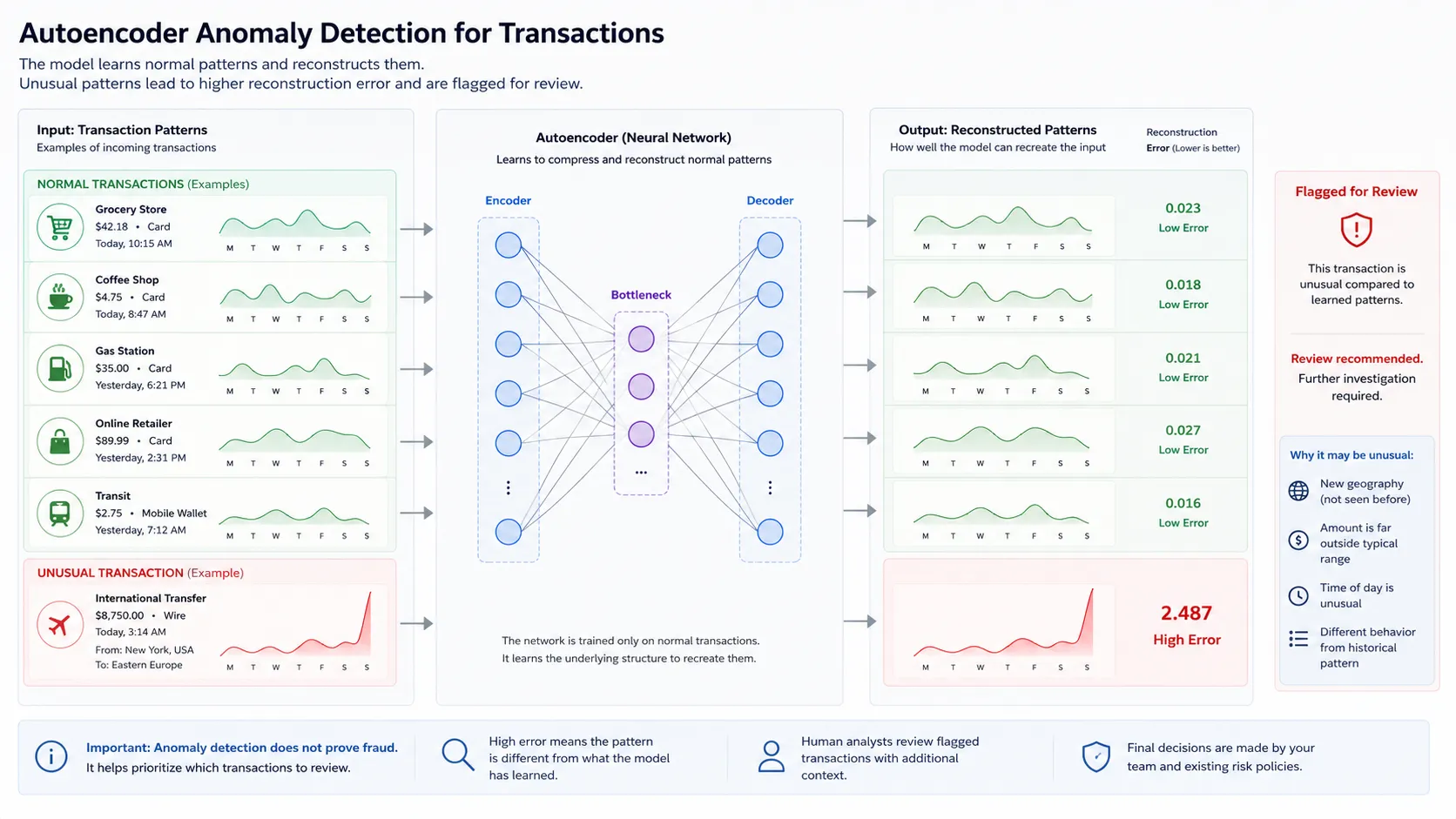
Now imagine a payment platform processes millions of transactions.
Most customers follow fairly normal spending patterns.
They may buy groceries, pay bills, order food, or shop online.
An autoencoder could be trained on patterns representing normal transactions.
The input could include features such as transaction amount, time, frequency, merchant type, or other relevant numerical information.
Suppose a new transaction appears with a pattern that is very different from what the model normally sees.
The autoencoder may reconstruct that transaction poorly.
Its reconstruction error rises.
The system can then send the transaction for additional fraud checks.
Again, the autoencoder is not directly saying:
“This transaction is fraud.”
It is saying:
“This transaction looks unusual compared with the normal patterns I learned.”
That makes autoencoders useful when unusual cases are rare and difficult to label.
Where Autoencoders Are Used
Autoencoders can be useful in several types of problems.
Image Denoising
A denoising autoencoder can learn to reduce unwanted noise while trying to preserve useful visual information.
This can help with scanned images, photographs, documents, and other visual data.
Anomaly Detection
Autoencoders can identify unusual patterns by measuring reconstruction error.
This can be useful for machine monitoring, sensor data, network activity, and some fraud-detection workflows.
Feature Learning
The encoder learns a compact representation of the input.
These learned features may be useful for other machine-learning tasks depending on the problem.
Dimensionality Reduction
Large datasets may contain many input features.
An autoencoder can create a smaller latent representation that captures useful information from those features.
This idea is related to dimensionality reduction, although autoencoders and traditional techniques such as PCA work differently.
Advantages of Autoencoders
One major advantage is that autoencoders can learn useful representations without requiring a class label for every input.
That can be valuable because labelled data is often expensive or difficult to collect.
Another benefit is flexibility.
Autoencoders can be designed for images, numerical data, signals, and other data types.
They can also learn nonlinear relationships.
This allows them to capture patterns that may be difficult to represent using simpler linear methods.
Denoising autoencoders have another useful property.
Because they learn to reconstruct clean information from corrupted input, they are encouraged to focus on stable patterns instead of blindly copying every detail.
Limitations of Autoencoders
Autoencoders are useful, but they are not a magic solution.
Their performance depends heavily on the training data.
If the training data does not represent the real problem well, the model may not learn useful patterns.
Anomaly detection can also be difficult.
Sometimes an unusual example may still be reconstructed well, which can make it harder to detect.
The opposite problem can happen too.
A perfectly normal example might receive a high reconstruction error simply because it is slightly different from the training data.
This can create false alarms.
Autoencoders can also require careful choices around architecture, latent-space size, training settings, and reconstruction-loss functions.
A bottleneck that is too small may remove useful information.
A model with too much capacity may become too good at reconstructing almost everything, including unusual data.
That can reduce its usefulness for anomaly detection.
When Should You Use an Autoencoder?
An autoencoder may be worth considering when you need to learn a compact representation of complex data, remove certain types of noise, or detect patterns that are different from normal training data.
For beginners, one of the best ways to understand autoencoders is to remember two questions.
For denoising:
“Can the model recover useful information from a corrupted input?”
For anomaly detection:
“Can the model reconstruct normal data better than unusual data?”
If those two ideas are clear, you already understand the core logic behind many practical autoencoder applications.
Final Thoughts
Autoencoders may sound complex when you first hear terms such as encoder, decoder, latent space, bottleneck, and reconstruction error.
But the central idea is surprisingly simple.
The encoder learns how to represent important information.
The decoder tries to rebuild the original data.
A denoising autoencoder learns to recover clean information from noisy input.
And an anomaly-detection autoencoder can use reconstruction error to find patterns that look different from what it learned as normal.
From restoring noisy images to monitoring machines and detecting unusual activity, autoencoders show how a neural network can learn useful structure without being given a traditional classification label for every example.
The best way to understand them is not to memorize definitions.
Instead, remember the journey:
Input → Encode → Compress → Decode → Reconstruct → Compare
Once that flow makes sense, autoencoders stop feeling like an advanced deep-learning mystery and start feeling like a practical tool you can actually understand and use.
Frequently Asked Questions About Autoencoders
What is an autoencoder in simple words?
An autoencoder is a neural network that learns how to represent data in a smaller form and then reconstruct it. It has two main parts: an encoder that compresses the input and a decoder that tries to rebuild it. Autoencoders are commonly used for feature learning, image denoising, dimensionality reduction, and anomaly detection.
How does an autoencoder work?
An autoencoder takes input data, passes it through an encoder, creates a compressed representation called the latent representation, and then sends it to a decoder. The decoder tries to recreate the original input. During training, the model compares the reconstructed output with the original data and improves by reducing the reconstruction error.
What is a denoising autoencoder?
A denoising autoencoder is trained using corrupted or noisy input while the clean version of the data is used as the target. This teaches the model to recover useful information instead of simply copying everything it receives. Denoising autoencoders are especially useful for learning robust features and reducing noise in images or signals.
What is the difference between an autoencoder and a denoising autoencoder?
A standard autoencoder normally receives clean data and tries to reconstruct that same data. A denoising autoencoder receives a corrupted version but is asked to reconstruct the clean original. Because of this, a denoising autoencoder learns to ignore some unwanted noise and focus on more stable patterns in the data.
What is latent space in an autoencoder?
Latent space is the internal representation created by the encoder. It contains a compact version of the important patterns the model has learned from the input. Instead of storing every original feature separately, the model represents useful information in this smaller feature space.
What is reconstruction error in an autoencoder?
Reconstruction error measures the difference between the original input and the output reconstructed by the autoencoder. A small reconstruction error means the model recreated the input closely. A larger error means the reconstructed output is more different from the original.
How is an autoencoder used for anomaly detection?
An autoencoder can be trained mainly on normal data so that it becomes good at reconstructing normal patterns. When unusual data is given to the model, reconstruction error may become higher because the pattern is different from what the network learned. A threshold can then be used to flag high-error examples as possible anomalies.
Can autoencoders be used for image denoising?
Yes. A denoising autoencoder can be trained by giving it noisy images as inputs and clean images as targets. Over time, the network learns to reconstruct cleaner versions by capturing useful visual structures while reducing some of the unwanted corruption present in the input.
What are the main applications of autoencoders?
Autoencoders are used for tasks such as image denoising, anomaly detection, feature learning, data representation, and dimensionality reduction. Different autoencoder architectures can also be adapted for images, signals, time-series data, and other types of information.
Is an autoencoder supervised or unsupervised?
Autoencoders are commonly described as unsupervised or self-supervised learning models because they do not require traditional class labels such as “cat,” “dog,” or “fraud.” Their training target is usually derived directly from the input itself, such as reconstructing the original clean data.
Autoencoder vs PCA: what is the difference?
Both autoencoders and PCA can create lower-dimensional representations of data, but they work differently. PCA is primarily a linear dimensionality-reduction technique, while neural-network autoencoders can learn nonlinear relationships when their architecture and activation functions allow it. Which one is better depends on the dataset and the problem being solved.
Why are autoencoders useful for anomaly detection?
Autoencoders are useful when normal examples are much easier to collect than abnormal ones. A model trained on representative normal data may reconstruct familiar patterns well while producing larger errors for unfamiliar patterns. Those reconstruction errors can then help identify observations that deserve further investigation.


