


Principal Component Analysis (PCA) Explained for Beginners
Imagine opening a dataset with 100 columns. At first, more information sounds better. Then you notice that many columns are telling almost the same story. A person’s monthly income may be closely related to yearly income. A car’s engine size may be connected with horsepower and fuel use. In a health dataset, weight and body measurements may carry overlapping information.
Your machine learning model still has to process every feature, even when several of them repeat similar patterns.
This is where Principal Component Analysis, or PCA, becomes useful.
PCA helps us represent a dataset with many features using fewer new features while trying to keep the most useful variation in the data. It is one of the most popular dimensionality reduction techniques in machine learning, but beginners often find it difficult because many explanations jump directly into covariance, eigenvalues, and eigenvectors.
We will not start there.
First, let us make the idea clear in simple English.
What Is Principal Component Analysis?
Principal Component Analysis is a technique used to reduce the number of dimensions, or features, in a dataset.
Suppose you have data about thousands of cars. For every car, you record price, engine size, horsepower, weight, fuel consumption, top speed, length, width, and several other values.
Some features may be strongly related. Cars with larger engines may often have higher horsepower. Heavier cars may consume more fuel.
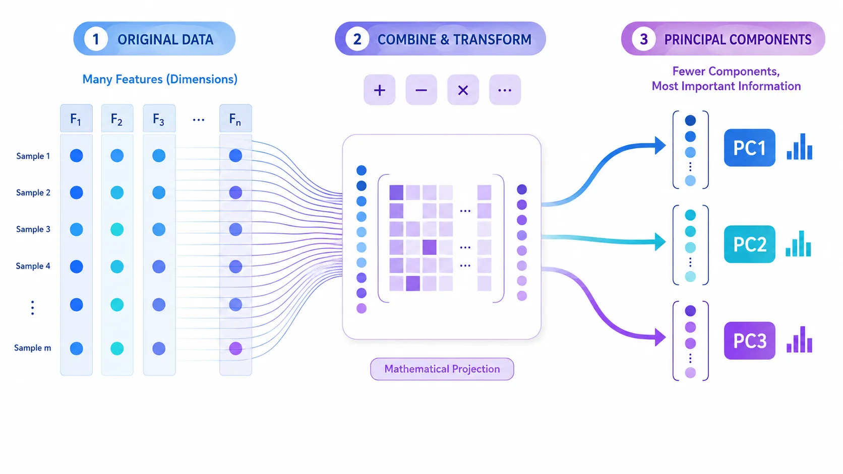
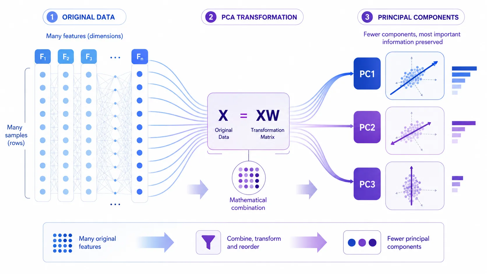
PCA studies these patterns and creates a smaller set of new variables called principal components.
These components are not simple copies of the original columns. Each one is built by combining information from multiple features.
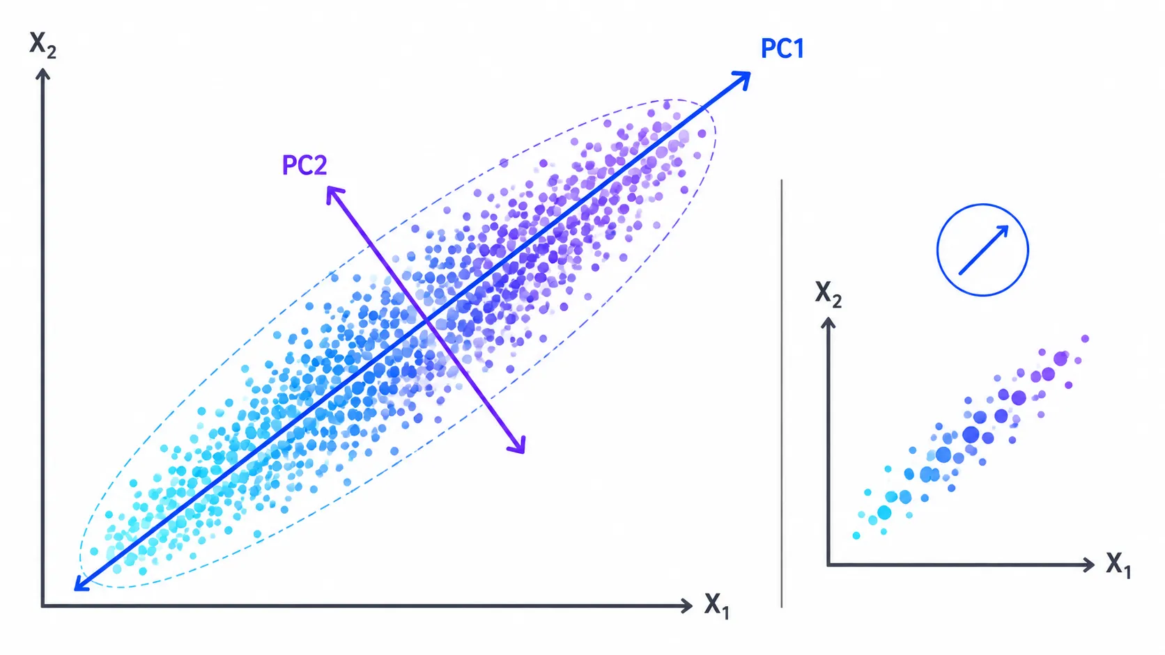
The first principal component, PC1, captures the direction where the data varies the most. The second principal component, PC2, captures the next most important direction without repeating PC1. The same idea continues with PC3, PC4, and so on.
The main idea is simple:
PCA tries to describe the important structure of a dataset with fewer dimensions.
If 20 original features can be represented well enough by 5 principal components, we may be able to work with those 5 components instead of carrying all 20 features into later analysis.
Why Do We Need Dimensionality Reduction?
A dataset with many features is called high-dimensional data. This is common in modern machine learning.
A small grayscale image with 100 × 100 pixels already contains 10,000 pixel values. A customer analytics system may track hundreds of actions for every user. A genetics dataset can contain thousands of measurements for one sample.
Too many dimensions can create real problems.
Too Many Features Can Slow Down Training
Every extra feature gives the model more data to process.
With millions of rows and hundreds of features, this can increase computation and make later analysis harder.
Reducing unnecessary dimensions can make the workflow simpler and often faster.
Some Features Carry Similar Information
Think about two columns: height in centimeters and height in inches.
They are technically different columns, but they contain almost the same information.
Real datasets often have less obvious versions of this problem. Several features may move together because they measure related things.
PCA can summarize these shared patterns instead of treating every correlated feature as completely separate information.
High-Dimensional Data Is Hard to Visualize
Humans can easily read two-dimensional and three-dimensional graphs.
We cannot directly visualize a dataset with 20, 50, or 500 dimensions.
PCA can project high-dimensional data into two or three principal components so we can inspect its overall structure on a normal plot.
A PCA plot can help us notice broad groups, unusual observations, or patterns that were difficult to see in the original feature space.
The Simplest Way to Understand PCA
Imagine a long pencil lying diagonally on a table.
If you look at it from a poor angle, it may appear shorter. From a better angle, you can see more of its full length.
PCA does something similar with data.
Instead of looking at the dataset only through its original axes, PCA searches for new directions that show the greatest spread of the data.
Why does spread matter?
Because a direction where observations differ strongly usually contains more information about how those observations are separated from one another.
The direction with the greatest variance becomes the first principal component.
After finding PC1, PCA finds another direction that captures as much of the remaining variance as possible while staying separate from PC1. That becomes PC2.
A useful way to picture this is that PCA rotates the coordinate system until the new axes line up with the strongest patterns in the data.
The data points do not change.
We change the way we describe their positions.
A Real-Life PCA Example
Imagine an online store tracks every customer using 30 features: visits, pages viewed, products opened, time spent, cart additions, purchases, average order value, discount usage, searches, and more.
Some of these features will naturally be related.
Customers who visit more may also view more products. Customers who buy more may also have higher total spending.
Instead of studying all 30 columns separately, PCA may find a few broader patterns hidden inside them.
One component might mainly reflect overall engagement.
Another might represent buying activity.
A third might reflect discount-driven behavior.
But PCA itself does not name them “engagement” or “buying activity.”
Those are human interpretations made after checking which original features contribute strongly to each component.
That is an important point.
PCA is generally used as an unsupervised learning technique because it looks for structure in the feature data without needing a target label.
For now, remember this:
PCA takes many possibly related features, finds new directions that capture the most variation, and represents the data using a smaller set of principal components.
Once this intuition is clear, the next step is to understand how PCA actually creates those components using standardization, covariance, eigenvalues, eigenvectors, and explained variance.
How Does PCA Work Step by Step?
Now that we understand the basic idea, let us see how PCA works step by step.
At first, the process may look mathematical, but the logic behind it is not difficult. PCA mainly tries to answer one question:
In which direction does our data contain the most useful variation?
To find that direction, PCA goes through a few important steps.
Step 1: Start With the Original Features
Suppose we have a simple dataset containing information about students.
For every student, we record:
hours studied
number of practice questions solved
test preparation time
These three features may be connected.
A student who studies more hours may also solve more practice questions. A student who spends more time preparing may also study more regularly.
So even though we have three separate columns, some of the information inside them may overlap.
PCA tries to find this shared pattern.
But before it can do that properly, we usually need to prepare the data.
Step 2: Standardize the Features
This is one of the most important steps in PCA dimensionality reduction.
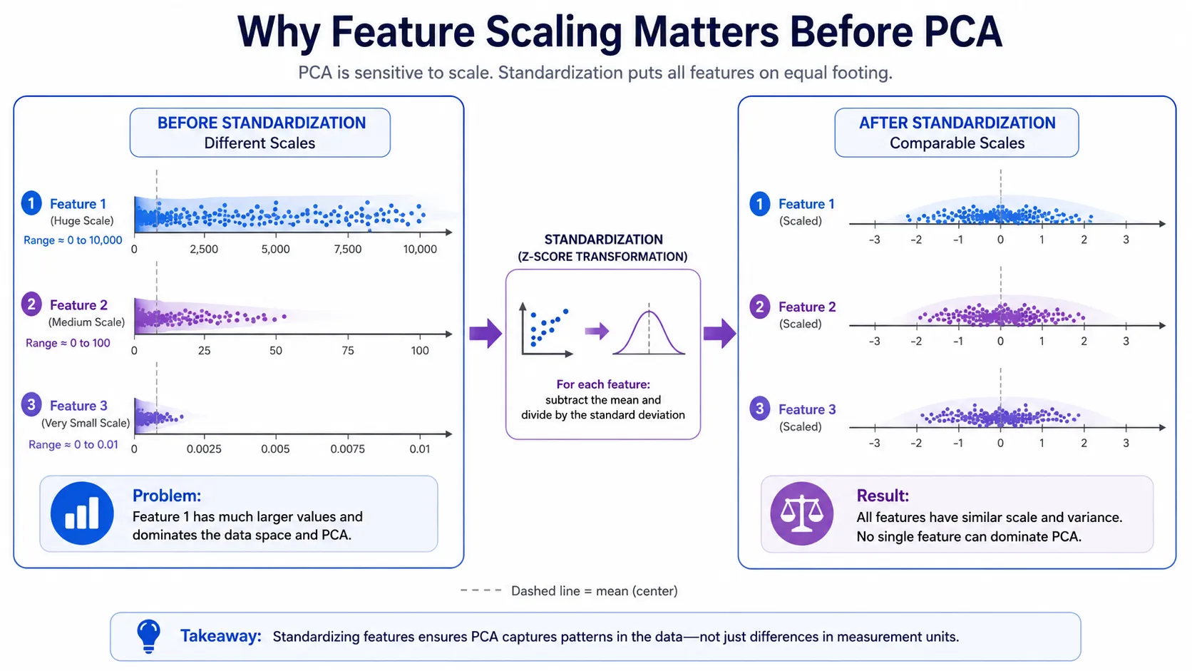
Imagine that one feature is annual income, with values such as 500,000 or 800,000, while another feature is age, with values such as 22, 35, or 50.
Income has much larger numbers than age.
If we apply PCA directly, the feature with the larger numerical scale may dominate the result simply because its values are bigger.
That does not automatically mean it is more important.
To avoid this problem, features are commonly standardized so they are measured on a comparable scale.
A standard value is often calculated using:
Standardized value = (original value − mean) / standard deviation
After standardization, each feature usually has a mean close to 0 and a standard deviation close to 1.
One small but important practical point: PCA implementations such as scikit-learn center the data before applying PCA, but PCA itself does not automatically scale every feature to the same variance.
So if your features use very different units, such as kilograms, rupees, centimeters, and years, scaling them before PCA is often important.
Step 3: Mean Center the Data
The next idea is called mean centering.
Suppose the average value of one feature is 50.
Instead of keeping values such as:
45, 50, 55
we shift them around zero:
-5, 0, 5
This does not change the relationship between the data points.
It simply moves the center of the data to zero.
Why do this?
Because PCA is interested in how data varies around its average position.
Once the dataset is centered, it becomes easier to find the directions where the data spreads the most.
Step 4: Understand Variance
To understand PCA properly, you need to understand variance.
Variance tells us how spread out the values of a feature are.
Imagine two classrooms.
In Classroom A, almost every student scores between 78 and 82.
In Classroom B, scores range from 35 to 98.
Classroom B has much higher variance because the scores are spread across a much wider range.
PCA pays a lot of attention to variance.
Why?
Because if a direction contains almost no variation, most observations look nearly the same in that direction. There is less information available to separate one observation from another.
A direction with larger variation can often tell us more about the overall structure of the dataset.
This is why the first principal component tries to capture the maximum possible variance.
Step 5: Find Relationships Using the Covariance Matrix
Now suppose we have two features:
hours studied and practice questions solved.
If students who study more also tend to solve more questions, both features increase together.
This relationship can be measured using covariance.
Positive covariance generally means two variables tend to move in the same direction.
Negative covariance means one tends to increase when the other decreases.
A covariance close to zero suggests that there may be little linear relationship between them.
When there are several features, PCA creates a covariance matrix that describes how the features vary together.
Do not let the word “matrix” make this feel complicated.
You can simply think of it as a structured way of asking:
Which features move together, and how strongly are they connected?
This information helps PCA find better directions for representing the dataset.
Step 6: Find Eigenvectors and Eigenvalues
This is usually the point where beginners think PCA becomes difficult.
You will often hear two terms:
eigenvectors and eigenvalues.
The names sound intimidating, but their role in PCA is easier to understand than the mathematics behind them.
What Is an Eigenvector in PCA?
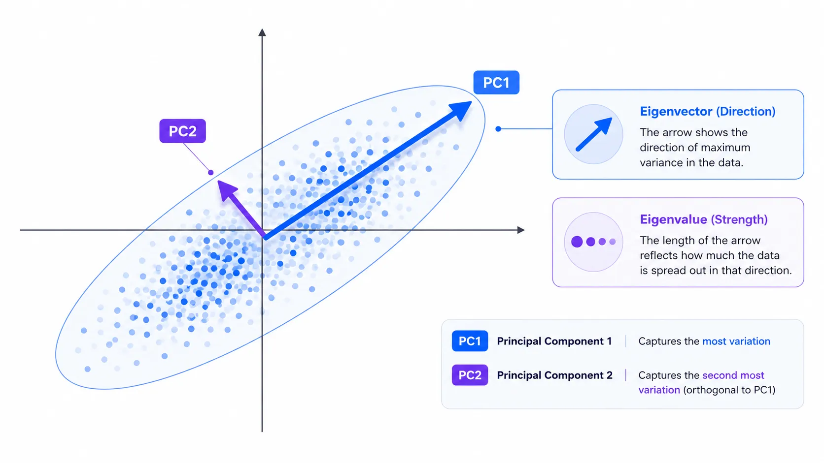
An eigenvector gives PCA a direction.
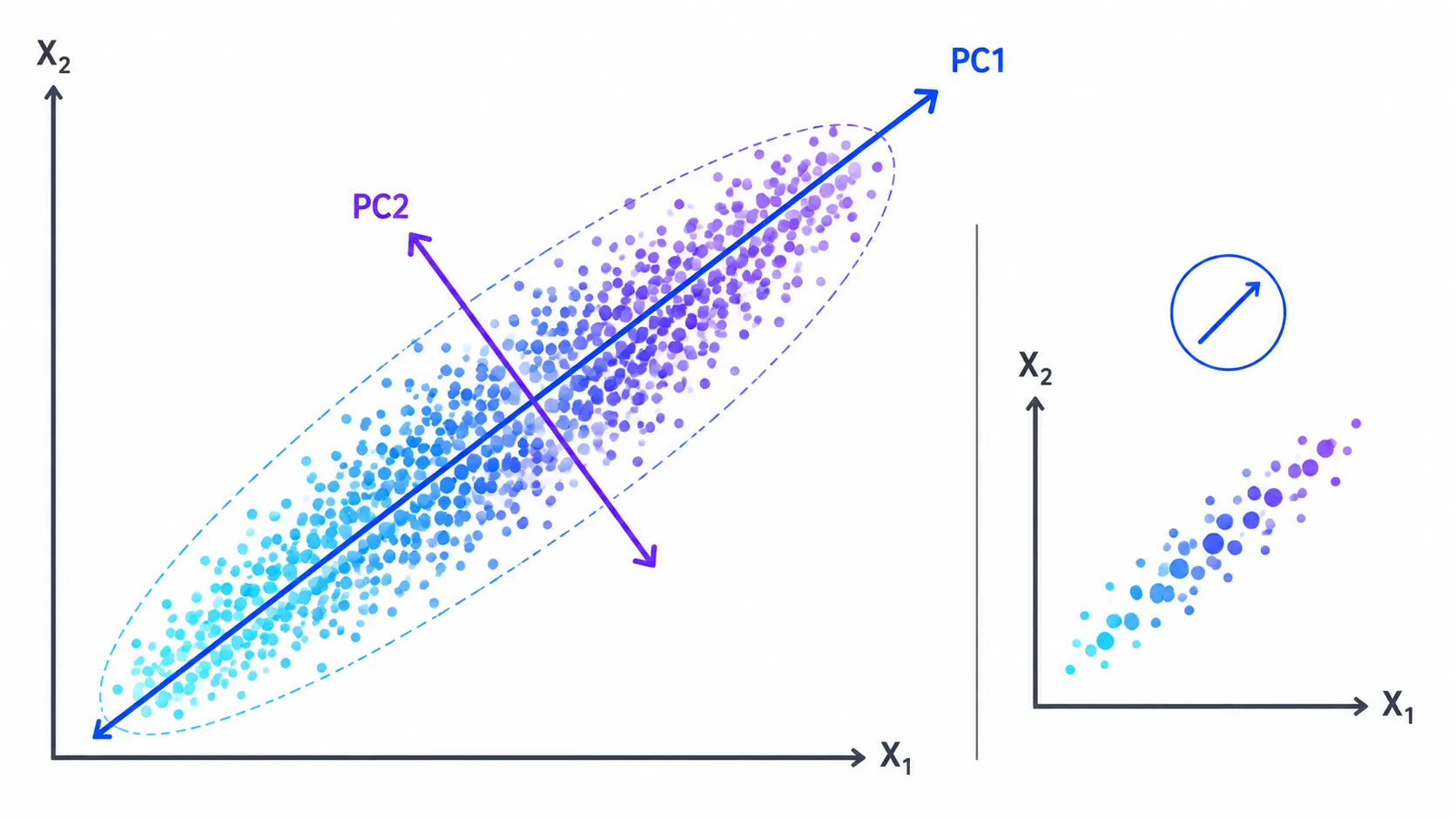
Imagine a group of data points forming a long diagonal cloud on a graph.
The longest direction of that cloud may be where most of the data variation exists.
An eigenvector helps describe that direction.
In PCA, these directions eventually become the principal component axes.
What Is an Eigenvalue in PCA?
If an eigenvector tells us the direction, the eigenvalue tells us roughly how much variance exists in that direction.
A larger eigenvalue means that direction captures more variation from the dataset.
A smaller eigenvalue means that direction captures less.
PCA sorts these directions from the largest eigenvalue to the smallest.
That is how it knows which principal components should come first.
So you can remember it like this:
Eigenvector = direction
Eigenvalue = importance of that direction in terms of variance
You do not need to manually calculate eigenvectors every time you use PCA in a machine learning project. Libraries such as scikit-learn perform the calculation for you.
But understanding what they represent helps you understand what PCA is actually doing.
Step 7: Create the Principal Components
After finding the important directions, PCA ranks them.
The first direction becomes:
Principal Component 1, or PC1
PC1 captures the largest amount of variance possible.
The next direction becomes:
Principal Component 2, or PC2
PC2 captures the largest amount of remaining variance while being perpendicular, or orthogonal, to PC1.
Then we can have PC3, PC4, and more.
Each principal component is created as a weighted combination of the original features.
For example, imagine a simplified component like:
PC1 = 0.60 × study hours + 0.58 × practice questions + 0.55 × preparation time
These numbers are only an example, but they show an important idea.
A principal component is not usually one original feature.
It combines multiple features into a new variable.
Step 8: Transform the Original Data
After the principal components are created, the original observations can be projected onto these new axes.
Suppose our original dataset had 10 features.
PCA might generate 10 possible principal components.
But we may discover that the first three components capture most of the useful variance.
Instead of keeping all 10 original dimensions, we can transform the dataset into just:
PC1, PC2, and PC3.
We now have a three-dimensional representation of the original ten-dimensional data.
This is the main idea behind feature reduction using PCA.
What Is Explained Variance in PCA?
Now we reach one of the most useful concepts in PCA:
explained variance.
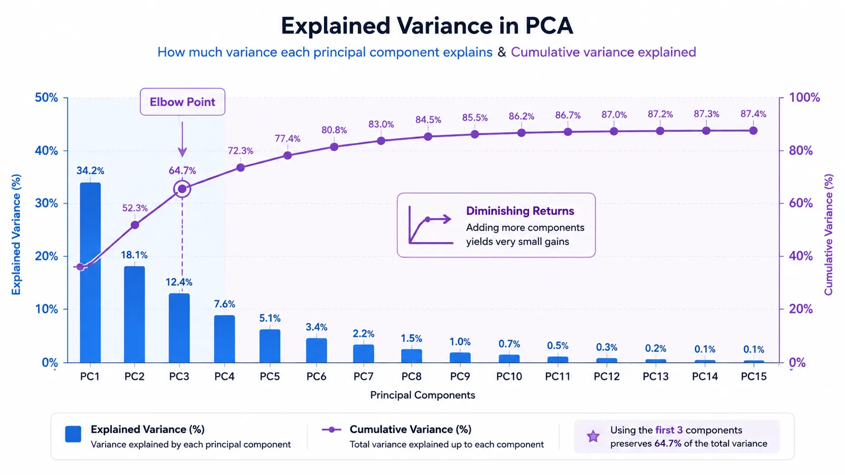
Explained variance tells us how much of the dataset's total variation is captured by each principal component.
Imagine:
PC1 explains 55% of the variance.
PC2 explains 25%.
PC3 explains 10%.
Together, the first three components explain:
55% + 25% + 10% = 90%
That means we may be able to represent the dataset using only three components while preserving around 90% of its original variation.
This leads to an important practical question:
How Many Principal Components Should You Keep?
There is no single number that works for every dataset.
Instead, we usually look at the cumulative explained variance.
For example, if:
2 components explain 70%,
4 components explain 90%,
and 8 components explain 98%,
then choosing 4 components may be a reasonable balance if 90% of the variance is enough for your project.
The right threshold depends on the problem.
Sometimes 90% is enough.
Sometimes a project may require 95% or more.
And sometimes keeping fewer dimensions is more valuable than preserving almost every small detail.
A common visualization called a scree plot can help us see how much variance each component explains and where adding more components starts giving smaller benefits.
At this point, we understand the complete logic behind PCA: prepare the features, center the data, study variance and covariance, find the important directions, rank them using eigenvalues, create principal components, and keep the components that preserve enough information.
The next important question is practical:
How do we actually apply PCA in Python, understand the output, and decide when PCA should or should not be used in a real machine learning project?
How to Apply PCA in Python
Once the idea behind PCA is clear, using it in Python is quite simple.
The most common approach is to use scikit-learn, which already provides a PCA implementation.
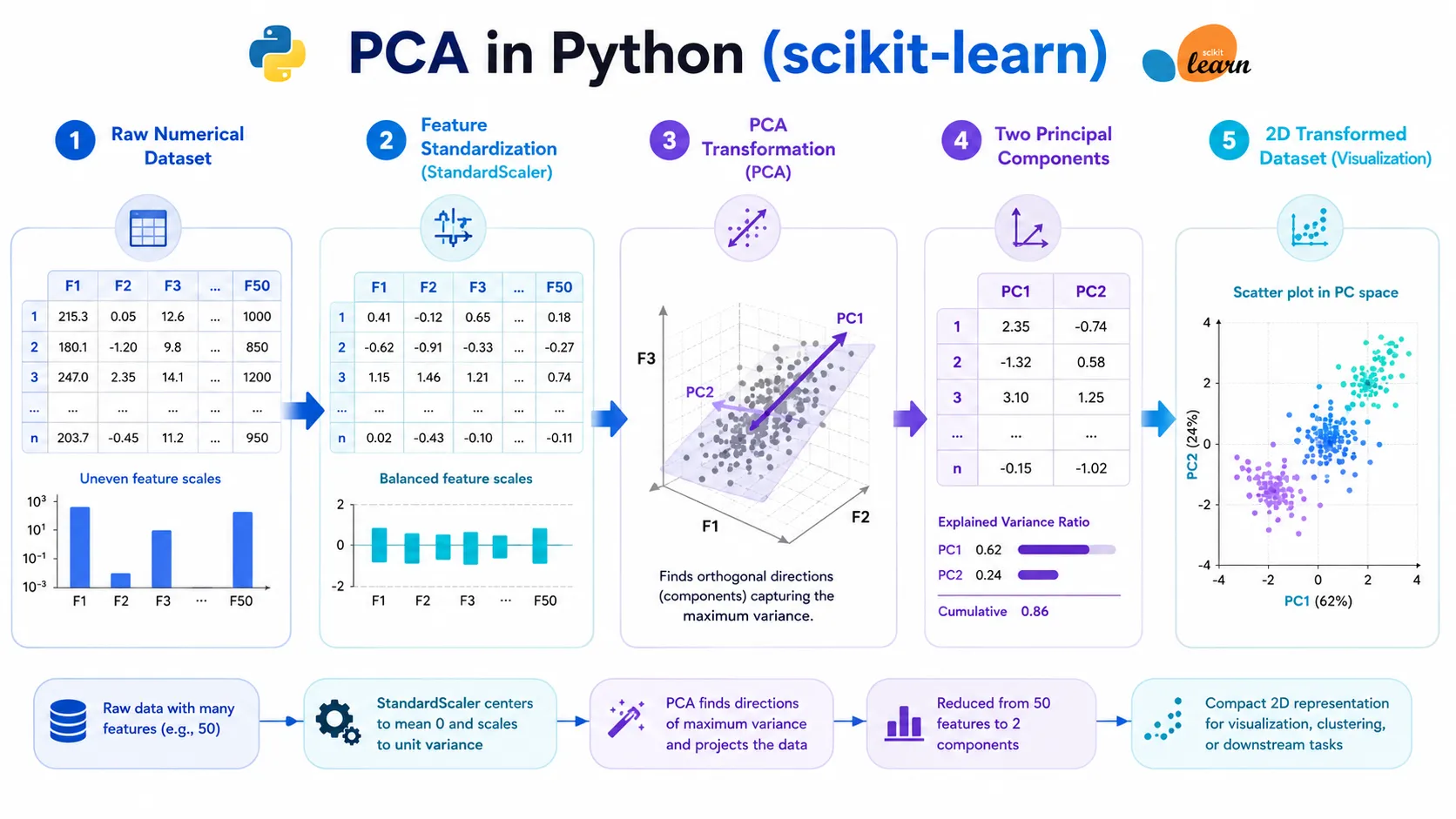
Before applying PCA, we normally separate the features, scale them when needed, and then decide how many principal components we want to keep.
Here is a simple example:
from sklearn.preprocessing import StandardScaler
from sklearn.decomposition import PCA
# Scale the features
scaler = StandardScaler()
X_scaled = scaler.fit_transform(X)
# Apply PCA
pca = PCA(n_components=2)
X_pca = pca.fit_transform(X_scaled)
print(pca.explained_variance_ratio_)
Let us understand what is happening here.
First, StandardScaler() puts the features on a comparable scale.
Then:
PCA(n_components=2)
tells PCA that we want to represent the original dataset using two principal components.
Finally:
fit_transform()
learns the important directions from the data and transforms the original observations into the new PCA space.
The result, X_pca, no longer contains the original feature columns.
Instead, each row is represented using PC1 and PC2.
A Simple Practical PCA Example
Imagine we have a customer dataset with 15 numerical features.
These may include:
number of website visits
products viewed
time spent on the website
cart additions
completed purchases
average order value
discount usage
number of searches
product reviews viewed
repeat visits
Several of these features may be connected.
For example, customers who visit frequently may also view more products and spend more time on the website.
After scaling the features, suppose we apply PCA and keep three principal components.
We may find that:
PC1 mainly receives strong contributions from website visits, products viewed, and time spent.
PC2 receives larger contributions from purchases and order value.
PC3 is influenced more strongly by discount usage and promotional activity.
We might interpret these components as broad patterns such as engagement, purchase behavior, and discount sensitivity.
But remember:
PCA does not automatically give these components meaningful names.
The names come from our interpretation of the feature contributions, often called PCA loadings.
This is why PCA is powerful but not always easy to explain.
What Are PCA Loadings?
PCA loadings tell us how strongly each original feature contributes to a principal component.
Suppose PC1 is strongly influenced by:
website visits, session duration, and products viewed.
That gives us an idea of what PC1 may represent.
If another component is strongly connected with order value and purchase frequency, it may represent buying behavior.
Loadings are useful when you want to understand what information each principal component is carrying.
However, we should avoid forcing a meaning onto every component.
Sometimes a principal component represents a mixture of several patterns that cannot be described with one simple label.
Using PCA for Data Visualization
One of the most common uses of PCA is high-dimensional data visualization.
Suppose your dataset has 50 features.
You cannot draw a normal 50-dimensional graph.
But you can reduce those 50 dimensions to two principal components and create a 2D scatter plot.
Each point on that graph represents one observation.
For example, each point could represent:
a customer, a product, a patient, an image, or a machine.
If similar observations naturally appear close together after PCA, we may notice groups or patterns.
A simple PCA visualization can be created with:
import matplotlib.pyplot as plt
plt.scatter(X_pca[:, 0], X_pca[:, 1])
plt.xlabel("Principal Component 1")
plt.ylabel("Principal Component 2")
plt.show()
This type of graph is useful for exploring the dataset before building a model.
Where Is PCA Used in Real Life?
PCA is useful in many areas where datasets contain a large number of related features.
Image Processing
Images can contain thousands or even millions of pixel values.
PCA can reduce the number of dimensions needed to represent image information.
This idea has also been used in areas such as face representation and image compression.
Customer Analytics
Businesses may track hundreds of customer actions.
PCA can summarize these variables into fewer components, making customer behavior easier to analyze.
Finance
Financial datasets may contain many related indicators, prices, or economic variables.
PCA can help identify common patterns that explain a large part of the movement in the data.
Biological and Medical Data
Datasets in genetics and medical research can contain thousands of measurements.
PCA is often used during exploratory analysis to reduce dimensions and visualize broad patterns.
Machine Learning Preprocessing
PCA can also be used before training another machine learning algorithm.
Reducing the feature space may make the next model easier or faster to train.
But PCA should not be applied automatically to every dataset.
Advantages of PCA
PCA offers several useful benefits.
It Reduces the Number of Features
A dataset with hundreds of features may sometimes be represented with far fewer principal components.
It Can Reduce Redundant Information
When several numerical features are strongly related, PCA can combine their shared variation.
It Helps Visualize Complex Data
Reducing data to two or three components makes it possible to create simple plots from high-dimensional datasets.
It Can Make Some Workflows Faster
Using fewer dimensions can reduce the amount of data later algorithms need to process.
It Can Help With Multicollinearity
Principal components are orthogonal to one another, so the new components are not linearly correlated in the same way many original features may be.
Limitations of PCA
PCA is useful, but it also has important limitations.
Principal Components Are Harder to Explain
Suppose your original features were age, income, and spending.
Those names have clear meanings.
After PCA, your model may instead use PC1, PC2, and PC3.
These components are combinations of the original features, so explaining them to a non-technical person can be harder.
PCA Is Sensitive to Feature Scale
If one variable has much larger numerical values than another, it may dominate the PCA result.
That is why feature scaling before PCA is often important.
PCA Mainly Captures Linear Structure
Standard PCA searches for linear combinations of the original features.
If the most important structure in your data is strongly nonlinear, PCA may not capture it well.
Some Information Is Lost
Dimensionality reduction usually involves a trade-off.
When we remove lower-variance components, we also remove some information.
The goal is not to keep everything.
The goal is to keep enough useful structure while making the dataset simpler.
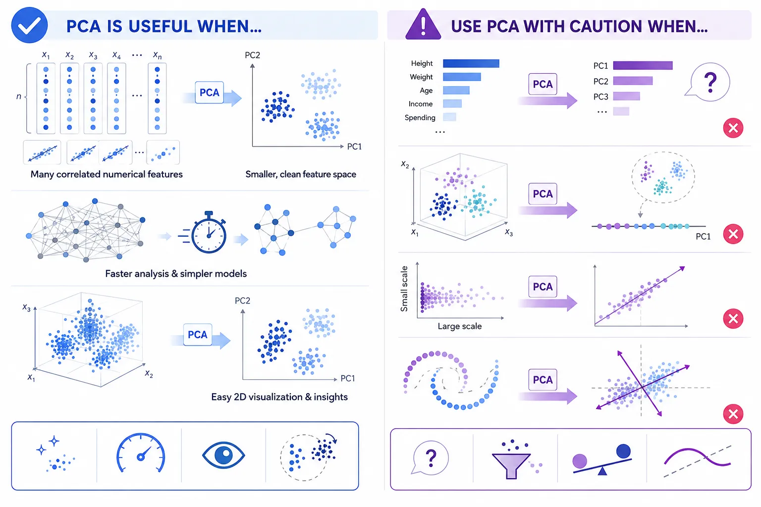
When Should You Use PCA?
PCA may be worth trying when:
your dataset contains many numerical features
several features are strongly correlated
you want to visualize high-dimensional data
you want to reduce the size of the feature space
model training is becoming expensive
you want to remove some redundant variation before later analysis
When Should You Avoid PCA?
PCA may not be the best choice when every original feature needs to remain easy to explain.
For example, imagine a bank must explain why a customer was rejected for a loan.
Saying that “PC4 had a large influence” is much less meaningful than saying that income or debt level had an influence.
PCA may also provide little benefit when your dataset already contains only a few useful features.
Common PCA Mistakes Beginners Should Avoid
One common mistake is applying PCA without checking feature scales.
Another is choosing principal components only because a certain percentage, such as 95%, sounds good.
The correct number depends on your actual problem.
A third mistake is assuming that a feature with low variance is always useless.
Low variance does not automatically mean that a feature has no predictive value.
Also remember that PCA does not look at the target variable when finding its components.
A direction with high variance is not automatically the direction that gives the best prediction for your target.
That distinction is especially important when PCA is used before supervised machine learning.
Final Thoughts
Principal Component Analysis may look complicated when we first see words like covariance matrix, eigenvalues, eigenvectors, explained variance, and principal components.
But the basic idea is surprisingly simple.
Imagine your dataset contains many different directions of information.
PCA looks for the directions where the data varies the most, ranks those directions, and allows us to keep the most useful ones.
Instead of working with a large number of original features, we can sometimes describe much of the same data structure using only a few principal components.
The most important thing is not memorizing every PCA formula.
Understand the flow:
prepare the data → find important directions → measure their variance → create principal components → choose how many to keep → transform the dataset.
Once that logic makes sense, the mathematics becomes much easier to learn.
And more importantly, you will know when PCA actually solves a problem instead of applying it simply because it is a popular machine learning technique.


